Excel Spreadsheet Basics
Excel is a spreadsheet program. A spreadsheet is a rectangular grid of cells. Each cell can contain a number, a formula or text. The value of a cell can depend on the values of other cells. If the value in any cell is changed, all the other cells are immediately updated to reflect that change.
Excel also has powerful built-in programming language called Visual Basic, which is described in another page.
You can start up Excel with a blank worksheet and follow the examples in this page, or you can download this spreadsheet and save yourself some typing.
Contents of this page
- Selecting, copying and moving cells
- Relative, absolute, and mixed references to cells
- Making graphs in Excel
- Solving equations numerically with Excel
- Doing matrix arithmetic with Excel
Selecting Cells
Excel works on the “Select, then do” principle. This means that you first select some cells, then you do something to them. For example you can select a cell and then start typing to enter something into the cell.
Selecting a cell. This is done by clicking your mouse near the center of the cell. Try selecting cell B2. The cell changes appearance. Cell B2 is now surrounded by a green box and in the lower right corner is a tiny square called the fill handle.

To select several cells in a rectangular block click and drag the mouse diagonally from one corner of the block to the opposite corner. Try selecting cells B2 to D3. Excel calls this a range and denotes it as B2:D3.

You can now enter data into this range by typing and pressing the Tab key to move from one cell to the next.
You can also select a non-rectangular range of cells by holding down the Control key (labeled Ctrl) while you select the cells. As before, you then press Tab to move from one selected cell to the next. Try selecting cells B2, D2 and E3:

You can also select an entire row, an entire column, several rows,
several columns or even the whole worksheet by clicking on the
row’s number, the column’s letter, or the gray triangle
![]() where they meet. For example here we selected row 2 and then made its
fill color yellow using the Fill Color tool
where they meet. For example here we selected row 2 and then made its
fill color yellow using the Fill Color tool
![]() .
Then we did the same thing to column D.
.
Then we did the same thing to column D.

Cells and Cell References
The cells of an Excel worksheet can hold text, numbers, dates, times or formulas. Excel looks at what you type and converts the cell contents as appropriate. If you type in a number, Excel stores it as a numerical value and you can use it for calculations. If you type in text (or a mixture of text and numbers), Excel stores it as text. If you type in something beginning with an equal sign (=) then Excel stores it as a formula.
Every cell has three properties associated with it: its content, its value and its format. The content is what you type into a cell, the value is what is displayed and the format is how it is displayed.
Example 1: Select the three cells A1, C2 and E3 (by holding down the Ctrl key). Type the number 5 into cell A1, press Tab, type the number 12 into cell C2, press Tab, and type the formula =A1+C2 into cell E3. Here is the resulting display:

Notice that although the content of cell E3 is the formula =A1+C2, the value is 17. Try changing either of the numbers in cells A1 or C2. The value in cell E3 is instantly updated. We say that cell E3 contains a cell reference to cells A1 and C2. Experiment with changing the format of cells A1, C2 and E3 using the tools on the Home Tab, shown here:

Moving Cells
To move a cell or range of cells, first select it and then move
the mouse pointer to the green boundary surrounding it.
When the pointer changes to a 4-way arrow,
![]() ,
click the boundary and drag the cell or range of cells to its new location.
,
click the boundary and drag the cell or range of cells to its new location.
Excel assumes that when you move cells you want to merely rearrange the spreadsheet but do not want to change its logic. Thus moving any cell causes all cell references to be updated accordingly.
Example 2: Continue from the previous example (where we had the number 5 in cell A1, the number 12 in cell C2 and the formula =A1+C2 in cell E3). Move the three cells to the locations shown below. Take a look at the contents of the cell A1. It still contains the formula, but that formula refers to the new locations of the numbers 5 and 12.

Copying Cells
There are several ways to copy a cell or range of cells. One way is to select the cells to be copied and then press Ctrl-C. Then select the destination cell or cells and then press Ctrl-V to paste them. Another way is to select the cells to be copied, then move the mouse pointer to the green boundary surrounding the cell. When the pointer changes to a 4-way arrow, press down on the right mouse button and drag the cell or range of cells to its new location. When you let the button go a pop-up menu appears giving you the choice of copying the cells, moving them, copying their formatting, etc. In all office products (Word, Excel, etc.) the right mouse button is programmed to bring up a context-sensitive menu and is a real time-saver.
Excel assumes that when you copy, you want any cell references in the copy to be relative to the new location in the same way that the cell references in the original were relative to the old location, as this example shows:
Example 3: Start from the previous example (which had the formula =C1+B1 in cell A1, the number 12 in cell B1, and the number 5 in cell C1). Select all three cells A1:C1 and press Ctrl-C to copy them. Now select cell A3 and press Ctrl-V to paste them. Here is the result:
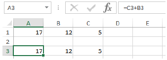
Notice that cell A3 now contains the formula =C3+B3, and not the formula =C1+B1. This is because Excel assumes that what you want to copy is the idea of adding the two numbers just to the right of the cell containing the formula.
Using the Fill handle to Automate Copying
The fill handle is the small box in the bottom, right corner of a selected cell:
This handle is used to fill neighboring cells in various ways using the selected cell or cells as a guide. Start with a fresh worksheet and try the following experiments:
- Type the number 5.5 into cell B1 and press Enter. Select cell B1. Click its fill handle and drag downward or across. The selection expands either down or across and the number 5.5 is repeated in all the dragged cells.
- Undo the above operation so that the number 5.5 is again only in cell B1. This time hold down the Ctrl key, then click in the fill handle and drag downward or across. This time the number 5.5 is incremented by one across the selected cells, i.e. 5.5, 6.5, 7.5, …
- Start with a fresh worksheet. Type 5.5 into cell B1 and 5.9 into cell B2. Select both cells, click on the fill handle and drag downward about 10 cells. The pattern of incrementing by 0.4 is propagated.
- Start with a fresh worksheet. Type the number 1 into cell A1, the number 1 into cell B1 and the formula =A1+B1 into cell C1. Now select cell C1 and click on its fill handle and drag across to cell K1. This produces the so-called Fibonacci sequence:

Notice that the formula in each cell sums up the values in the two cells to the left of it. For example, cell K1 contains the formula =I1+J1.
Relative, Absolute and Mixed References
The cell references used so far are called relative references because they refer to positions relative to the present position. They make it easy to apply a formula to an entire list of values as in the example above. Another type of reference is the absolute reference. An absolute cell reference does not change when you copy a formula. To make a cell reference absolute, type a $ sign before the column and before the row. For example $B$1 is an absolute reference to cell B1.
Example 4: Suppose that we wish to make a table of values for the function y = a x 2, for integer values of x from −2 to 2. Also suppose that presently the ‘parameter’ a equals 5 but that this value may change in a later example. The most efficient way to do this is to put the value of parameter a into, say, cell A1 and the x values into, say, column D and then put the formula =A1*D2^2 into cell E2.

Tip: In the picture above the blue arrows show where cell E2 gets its value. The arrows can be displayed by going to the Formulas tab and in the Formula Auditing group clicking on Trace Precedents. The arrows can be removed by clicking the Remove Arrows button just below it.
To finish our table of values we might expect that we could select cell E2 and drag its fill handle downward to propagate its formula to the other cells in column E. But this does not give the desired result as we see here:
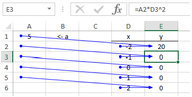
The blue arrows show what is wrong. We want the formulas in column E to all refer to the number 5 in cell A1 but they don’t. Why? Because when cell E2 is copied downward, its reference to cell A1 becomes a reference to cell A2, A3, etc. which are blank.
This is the way Excel works by default. We need to force Excel to use cell A1 for all the cells in column E.
To do this we change the reference in cell E2 from A1 to $A$1. This is called an absolute reference. The result of doing this and then copying is exactly what we want:
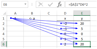
It is also possible to make the column relative and the row absolute or vice versa in a cell reference. In the above example we could have made the formula in cell E2 read =A$1*D2^2 (making only the row absolute) and the copying would have also worked as desired. This is called a mixed reference.
Example 5: Let’s do an experiment that shows how all the possible combinations of absolute and relative references work when they are copied. Start with a fresh sheet and type the number 5 into cell A1 and type the eight formulas into the eight cells as shown here:

Of course you don’t actually see these formulas – you see the resulting values displayed, like this:

There is a Show Formulas button that you can use to toggle the display back and forth to
either show the formulas or to show the resulting values.
This button is in the Formulas tab in the Formula Auditing group
and looks like this:
![]()
Now we will do some copying.
- Select the four numbers in column E and drag the Fill Handle to the right by one column.
- Next, select the four numbers in row 5 and drag them down by one row.
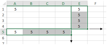
Here is the result of the copying. (We have colored the cells to make it easier to explain what happened. Red fill means that the reference to cell A1 did not change and green fill means that the reference did change.)

If we use the ![]() button
to look at the formulas we see this:
button
to look at the formulas we see this:

Notice that:
- The relative reference A1 changes when copied in either direction.
- The absolute reference $A$1 doesn’t change when copied in either direction.
- The mixed referenced A$1 doesn’t change when copied downward (because the row (1) is absolute) but does when copied across (because the column (A) is relative).
- The mixed referenced $A1 doesn’t change when copied across but does when copied downward.
Tip: A shortcut for toggling an existing cell reference from relative
→ absolute → mixed is to select it in the Formula Bar and then
repeatedly press the F4 key. (The Formula Bar is the box to the right of
![]() .) Here is a picture:
.) Here is a picture:
Before:

After:

Making Graphs
The most useful type of graph (or chart in Excel lingo) for mathematical and engineering applications is the X-Y Scatter graph. (This is the only type of Excel chart that allows x values to be entered together with y values.) The steps are:
- Create the table of values to be graphed.
- Select the table of values (including any headings).
- In the Insert tab, Charts group, click on the scatter type to create the rough graph.
- Choose various options to make the graph look just right.
Example 6: Graph the trigonometric function y = 100sin(x) + 50cos(2x) between x = 0 and x = 2π.
The first step is to create a table of values for the graph. The x values will be in column B and the y values will be in column C. The table will have 42 rows: the headings in row 1 and the values in the following 41 rows. These are enough values to produce a nice, smooth curve. We want the x values to run uniformly from 0 to 2π and the easiest way to do this is to use an index n. We can let n run through the integers 0, 1, 2, … 40 and use the formula x = n π / 20. This will cause x to run from 0 to 2π in 40 equal increments.
Start the table by entering the following text, numbers and formulas into the seven cells shown:

The cells in row one are just text and are the headings. Column A will eventually contain the index numbers n from 0 to 40. Cell B2 contains the formula that gives the x value in terms of the index n. PI() (with nothing in the brackets) is a built-in function in Excel that gives the value of π to 16 decimal places. Cell C2 contains the formula that gives the y value as a function of x. SIN(x) and COS(x) are also built-in functions. Note that their argument, x, cannot be in degrees – it must be in radians.
Now we can fill in the rest of the table using the Fill Handles. First, select the range A2:A3 as shown below and drag the fill handle downward. A tiny “indicator box” appears showing the value of n so far. Continue until n = 40. This is the bottom of the table of values. Second, select the range B2:C2 as shown below and double-click on the fill handle. Double-clicking is a great shortcut that copies the selected column or range downward as far as the previous column. The table of values is complete.

We are now ready to draw the graph. Select the table of values. Include the headings but not the index column (i.e. select the range B1:C42). Then click on the Insert tab and in the Chart group click on Scatter. There are five scatter types. Let’s click on the third one – smooth lines and no markers:
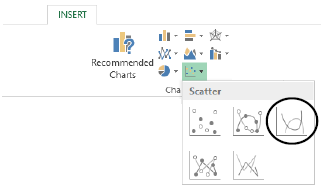
The result is the graph shown below. It is a bit rough and needs some formatting. To format the graph, click on it. Three things happen.
- The graph is selected. You can click on elements like the title, gridlines and axes right in the graph to move, format or delete them.
- The table of values is selected (colored boxes appear around the x range, the y range and the heading and ‘resizing handles’ appear on them). You can move them or change their length to change the data being graphed.
- Three buttons appear to the right of the graph. They open dialog boxes that gives you even greater control in formatting the graph elements. The third button allows you to add more curves to the same graph.

Here is the result of making some changes to the axes, gridlines and colors.
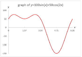
Tip: A quick way to plot two curves on the same graph (what Excel calls two data series) is to create a table of values with an x column and two y columns. Give each y column a heading. Select all three columns and then click on Insert, Charts, Scatter. The headings are put into a legend below the graph as shown here:
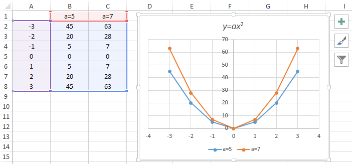
Another tip: You don’t always have to use an index. (In the graph above we didn’t use one.) Also you can let x have any values you want. If your graph is changing more rapidly in a certain region of x then you can insert a few extra rows in your table of values and let the x values be more closely spaced in those rows. If you insert a blank row in your table of values then the graph will have a break in it.
Another tip: If you want to create a polar plot then first make a table of values of the radius r and the angle θ and then use the formulas x = r cos(θ) and y = r sin(θ) to get x and y. Then plot the x and y columns in a scatter graph.
Example 7: Use markers to plot the set of points with polar coordinates
{r = ![]() , θ = 2.4 n},
where the index n is an integer running from 0 to 500.
These equations come from a study of how sunflower seeds arrange themselves in a sunflower.
, θ = 2.4 n},
where the index n is an integer running from 0 to 500.
These equations come from a study of how sunflower seeds arrange themselves in a sunflower.
Set up the headings in row 1 and the formulas in row 2 as shown here:

Then fill out column A with the numbers 0 to 500. Then select the four cells shown above and double-click the fill handle. The table is now completely filled in. Select columns D and E and click on Insert, Chart, Scatter (with markers only). Here is the result after some formatting – a beautiful spiral pattern similar to the arrangement of seeds in a sunflower:
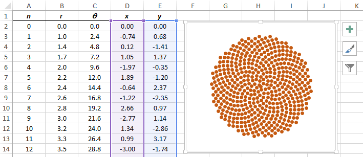
Let’s explain this picture. The pair of equations
{r = ![]() , θ = 2.4 n},
describe a spiral because both the radius and the angle increase with n.
, θ = 2.4 n},
describe a spiral because both the radius and the angle increase with n.
The radius formula is designed so that the markers (sunflower seeds) maintain a
uniform density no matter how many there are (recall the circle area formula
A = π r 2 so
the number of markers per unit area is constant if we let
n ∝ r 2 or r ∝
![]() ).
).
The angle formula is the result of arguments that have to do with the
golden ratio φ.
(φ ≈ 1.618..., so ![]() ).
One important thing is that the angle changes so rapidly (by 2.4 radians or 138°
with each successive marker) that the spiral is impossible to see from just looking
at the markers. Therefore let's make another graph. Let’s superimpose the markers
on the spiral. We do this by putting two data series on the same graph.
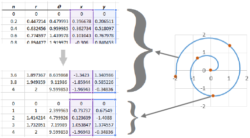
The first data series has n going from 0 to 4 in increments of 0.2 and is
formatted to give the smooth blue curve with no markers. The second data series has
n running through the integers 0, 1, 2, 3, 4 and we formatted this one to
give brown markers with no curve. Here is the graph:
).
One important thing is that the angle changes so rapidly (by 2.4 radians or 138°
with each successive marker) that the spiral is impossible to see from just looking
at the markers. Therefore let's make another graph. Let’s superimpose the markers
on the spiral. We do this by putting two data series on the same graph.
The first data series has n going from 0 to 4 in increments of 0.2 and is
formatted to give the smooth blue curve with no markers. The second data series has
n running through the integers 0, 1, 2, 3, 4 and we formatted this one to
give brown markers with no curve. Here is the graph:
Solving Equations Numerically with Excel
When we want to solve an equation like 5 x = 15 we generally try to use algebra. But there are many equations that are either difficult or impossible to solve with algebra. A simple example is the equation 2 x = 2 − x. Then we have to use a numerical method. This means that a computer simply tries many values of x until it finds one that satisfies the equation. Excel has two numerical methods to solve equations:
- Goal Seek, found in the Data tab, Data Tools group, What-If Analysis. It is very basic.
- Solver. This is an Add-in (i.e. it is not normally part of Excel) and is much more advanced than Goal Seek. To make it available, you must go to the File tab, Options, Add-Ins and at the bottom of the dialog box select Manage Excel Add-Ins and click on Go... In the dialog box that opens check the Solver Add-in box and press OK. When you go back to Excel you will find a new group under the Data tab called Analysis and this is where Solver is located.
Using Goal Seek
If we know the result that we want from a formula, but don’t know what input value the formula needs to get that result, then we can use Goal Seek. For example the graph above shows that when x = 0 then y = 50. But what if we want to know what value of x yields y = 70? Here is how we can find it using Goal Seek – essentially how we can solve the equation 100 sin(x) + 50cos (2x) = 70.
Enter any number into cell A2 (we have entered zero). Then enter the formula shown into cell B2.

Select cell B2. Then, in the Data tab, Data Tools group, click What-If Analysis, and then click Goal Seek. The dialog box shown to the right opens.
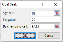
- The Set cell box already contains B2, the cell containing the formula, because we had selected it earlier.
- In the To value box, type the value that we want cell B2 to equal, namely 70.
- In the By changing cell box, enter the cell that needs to change to yield the number 70. Tip: The quickest way to fill in this box is to click on cell A2 in the spreadsheet.
- Click OK. After a moment we have the result: when x = 0.280039 then y = 69.99999.
You may see Goal Seek rapidly try several values before it stops at 0.280039 and decides that is close enough. You may also see that it finds a completely different solution if you start with a different ‘seed’ (initial x value). For example if you start with cell A2 containing 3.14 then Goal Seek finds the solution x = 2.861555 where y also equals 69.99994.
Using Solver
Like Goal Seek, Solver can solve equations. But in addition, it can solve systems of equations, solve inequalities, and it can minimize or maximize functions subject to constraints.
Example 8: The graph above shows that the curve y = 100 sin(x) + 50cos (2x) has a relative maximum somewhere between x = 1.57 and x = 3.14. Use Solver to find it to 10 decimal places.
First let’s make sure that we can see the 10 decimal places. Select cells A2 and B2. Then in the Home tab, Number group, click the arrow circled in the picture below to expand the Number group. Set the selected cells to show numbers to 10 decimal places.
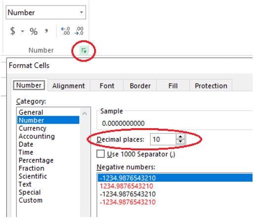
Now, as before, enter a seed number into cell A2 and the formula to be maximized into B2. (Any seed in the region between 1.57 and 3.14 will work. We have entered 2.)

Then, in the Data tab, Analysis group, click on Solver. The dialog box shown here opens. We must set all the parameters circled in red:
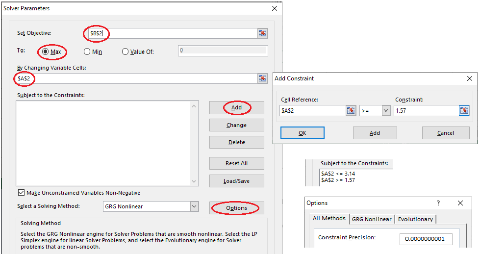
- The Objective and By Changing cells are exactly as in Goal Seek, i.e. B2 and A2.
- The To option to set to Max (note that ‘value of’ is then irrelevant).
- The Add button is used to add the two constraints x ≥ 1.57 and x ≤ 3.14.
- The Options dialog is where we set the calculation to an accuracy of 10 decimal places.
- Click OK. After a moment we have the result: when x = 2.6179938759 then we are at the local maximum value of y = 75.0000000000.
Try changing the constraints to find the other local maximum. (It is located at x = 0.5235987756.)
Example 9: Solve the following system of equations for x, y and z using Solver:

Note: In Example 10 we will solve this problem using a matrix method but here we will solve it by creating a function and using Solver to find the minimum of that function.
To understand the function that we are about to create, imagine that we simply try millions of combinations of x, y and z to find the solution. For example if we try {x = 1, y = 1, z = 1} then the equations read 16 = 80, −1 = 7, and 4 = 22, and we know that can’t be the right solution because the left-hand-side (lhs) must equal the right-hand-side (rhs) for each equation. Eventually we would try {x = 7, y = 5, z = 3} and then the equations would read 80 = 80, 7 = 7, and 22 = 22, meaning that we have found the right solution. Now consider the expression
The notation lhs1 means the left-hand-side of the first equation, etc. Each term describes how different the left and right sides are for one of the equations. Squaring makes all the terms positive. Adding the terms together means that all three equations are included in the expression. Notice that this expression is zero for the right solution and is positive for any wrong solution. We can make a function out of this expression. Because it depends on x, y and z the function is denoted like this:
We can use Solver to either find where this function is zero or to find where the function has its minimum. We use the word ‘where’ because we could imagine that we are searching in a 3-dimensional space that contains (x, y, z) points like (1, 1, 1) and (7, 5, 3).
Let’s start filling in the spreadsheet as shown in the picture below.
- Copy the numbers from the system of equations into columns A, B, C, and F.
- Put any values whatsoever for x, y and z into column D. They are seed numbers and Solver will change them.
- Enter the formula =A3*$D$3+B3*$D$4+C3*$D$5 into cell E3. This is lhs1. Drag its fill handle downward to copy the formula to the two cells below it. (Note that the copying works correctly because the references to D3, D4 and D5 are absolute references.)
- Put the formula =(E3-F3)^2 into cell G3. This is the first term of our function, namely (lhs1 − rhs1)2. Copy it downward two cells also. Finally put the sum formula shown into cell G6. This is our function. This is the cell that we want to minimize.

We will use Solver to change the values in D3:D5 and make the target cell G6 become a minimum. Start Solver and fill in the dialog box as shown:

Click on Solve, then on OK to close the dialog box. The answer is that our function takes on a minimum value of zero when {x = 7, y = 5, z = 3}.
Other things to try:
- Start with different seed values for x, y and z and verify that the solution is unchanged.
- Use Solver to find where the function takes on the value zero. Verify that the solution is again {x = 7, y = 5, z = 3}.

Matrix Operations
In this section we show how to use Excel to do matrix operations (scalar multiplication, addition, subtraction, multiplication, calculating the inverse, transpose and determinant).
Tip: Let's give the spreadsheet some formatting that is useful for matrices.
- First let's make all the cells square. Select the whole spreadsheet by
clicking on the triangle in the upper-left corner:

- Now move the mouse to the top of the spreadsheet where columns A and B
meet:
 .
When the cursor changes to
 ,
drag left. This decreases the width of all the columns.
- Do the same for rows. Move the mouse to where rows 1 and 2 meet
and when the cursor changes to
 ,
drag down to increase the height of all the rows.
- Center all cell contents both vertically and horizontally by
clicking these buttons (located on the Home tab, Alignment group):

Tip: If you want Excel to interpret the contents of a cell as a string of text instead of as a number or a formula then start the text with an apostrophe ('). Here are two examples:
- In the picture below we want a cell to display an = sign. The problem is that Excel interprets that as the beginning of a formula. To force it to be text, we must type in '=.
- ID numbers and telephone numbers are not numbers to do arithmetic on (i.e. you don’t add or subtract them). For example, if 00325 is supposed to be an ID number, and if you type 00325 into a cell, Excel will interpret it as a number and display it as 325. But if you type in '00325 it will be text and will display as 00325.
Tip: In the examples that follow we will give the matrices a fill color and a border to make them stand out. Also we will put *, =, +, – characters in cells only to make the intention of the example clear. Those characters are not necessary.
Multiplication of a Matrix by a Scalar
Here is an example. The scalar (number) is in cell B3 and the matrix is in the range D2:F4.
- Select the range where you want the product to go. We will use the range H2:J4. The selection must be the correct size to hold the product (3x3 for this example).

- Type in = to indicate the beginning of a formula.
- Select the scalar.
- Type in the multiplication symbol *.
- Select the matrix. At this point the formula bar shows = B3 * D2:F4.
- Hold down both the Ctrl and Shift keys and then press Enter. (Windows denotes this as CTRL+SHIFT+ENTER.) Here is the result:

Notice that if you select any cell in the resultant matrix the formula bar now reads {= B3 * D2:F4}. The braces indicate that the selection is part of an array formula. You cannot move or delete a part of an array. You must select the entire array H2:J4 and move it or delete it.
Tip: The above method of selecting the scalar and the matrix is much easier that the alternative of typing =B3*D2:F4 into the formula box.
Matrix Addition and Subtraction
Adding or subtracting matrices is very similar to the above.
- Select the range where the sum or difference is to go. It must be the same size as the matrices to be added.
- Type in = to indicate the beginning of a formula.
- Select the first matrix.
- Type in a + or – symbol.
- Select the second matrix.
- Hold down both the Ctrl and Shift keys and then press Enter. Here is an example:

The rest of the matrix operations – multiplication, calculating the inverse, transpose and determinant are done using functions (=MMult, =MInverse, =Transpose and =MDeterm).
Matrix Multiplication
- Select the range where the matrix product will go. It must be the correct size.
- Type in =MMult( to denote the beginning of the matrix multiplication function. This function takes two arguments: the left matrix and the right matrix.
- Select the first matrix.
- Type in a comma “,”
- Select the second matrix.
- Hold down both the Ctrl and Shift keys and then press Enter. Here is an example:
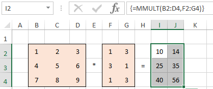
Tip: You don’t have to type in the closing bracket of =MMULT(B2:D4,F2:G4). Excel puts it in for you.
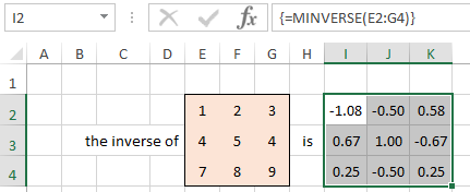
Matrix Inversion
This is also done using a function. To invert a matrix:- Select the range where the inverse will go. It must be the correct size.
- Type in =MInverse( to denote the beginning of the matrix inversion function.
- Select the matrix.
- Hold down the Ctrl and Shift keys and then press Enter. Here is an example:
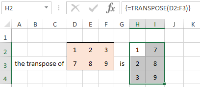
The Transpose of a Matrix
This is also achieved using a function. To transpose a matrix:
- Select the range where the transpose will go. The selection must be the correct size for the transpose.
- Type in =Transpose( to denote the beginning of the transpose function.
- Select the matrix.
- Hold down the Ctrl and Shift keys and then press Enter. Here is an example:
The Determinant of a Matrix
To calculate the determinant of a matrix:
- Select the cell where the determinant will go.
- Type in =MDeterm( to denote the beginning of the determinant function.
- Select the matrix.
- Hold down the Ctrl and Shift keys and then press Enter. Here is an example:

Example 10: Solve the following system of equations for x, y and z using matrix methods (i.e. by using the inverse matrix).

Solution: We can write these three equations as a single matrix equation.

Let’s give names to the three matrices.

Now the matrix equation can be written as A x = b, which can be solved to give x = A−1 b. Here is the Excel spreadsheet that first calculates the inverse, A−1, and then calculates the product, A−1 b, which is the solution x.

The solution in matrix form is  which means that
  .
.
If you would like to leave a comment or ask a question please send me an email!