Systems of Linear Equations and Gaussian Elimination
What is a System of Linear Equations?
A linear equation in n unknowns x1, x2, … , xn is an equation of the form:
a1 x1 + a2 x2 + … + an xn = b
where a1, a2, … , an and b are constants.
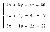
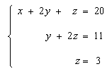
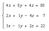
The name linear comes from the fact that such an equation in two unknowns or variables represents a straight line. A set of such equations is called a system. An example of a system of three linear equations in the three unknowns x, y and z is:
Some lessons to learn from graphing 2 equations in 2 unknowns
The graphical method is not very useful as a computational tool but it is useful for visualizing concepts such as the uniqueness of the solution or the meaning of inconsistent or redundant systems. Consider the following system of two linear equations in two unknowns:
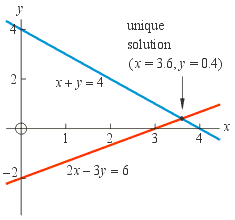
In this method we simply draw graphs of the equations as we have done to the right. Notice that the graph of each equation is a straight line. (This is the hallmark of a linear system. There are no curves, only straight lines.)
Any point on one line is a solution of one equation and any point on the other line is a solution of the other equation. The point where the lines cross {x=3.6,y=0.4} is the solution that satisfies both equations simultaneously. Notice that the solution is unique. This is because the lines are straight and there is only one point where they can cross.
A system of linear equations with a unique solution is the "normal" situation. However it is possible to have a system of equations with no solution. Such a system of equations is called inconsistent. It is often the result of an inaccurate or incorrect analysis of the physical system being described by the system of equations.
Consider the following system of two linear equations in two unknowns:

This system of equations is inconsistent because there is no way that x+y can equal 2 and 4 at the same time. The figure to the right shows that the graph of this system consists of two parallel lines that never cross. Thus there is no solution.
It is also possible to have a system of equations with an infinite number of solutions.
Such a system of equations is called redundant. It is often the result of an incomplete
analysis of the physical system.
Consider the following system of equations:
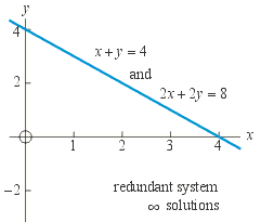
This system is redundant because the second equation is equivalent to the first one. The graph consists of two lines that lie on top of one another. They 'cross' at an infinite number of points, so there are an infinite number of solutions.
To summarize, a linear system with 2 unknowns must have at least 2 equations to get a unique solution. Having 1 equation is not enough, because 1 equation in 2 unknowns is represented by an entire line. Having 2 equations is exactly enough, as long as they are not redundant or inconsistent. Having 3 (or more) equations is too many. The third equation must be either redundant or inconsistent.
These ideas can be generalized to linear systems of equations with more unknowns:
A linear equation in n variables represents a "hyperplane" in an n dimensional space.
A linear system of equations with n unknowns must have at least n equations to get a
unique solution. Having any fewer is not enough; the solution will not be unique.
Having n equations is exactly enough, as long as they are not redundant or inconsistent.
Having any more than n equations is too many; the system will be either redundant or inconsistent.
The Augmented Matrix
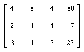
We will represent a system of equations by a rectangular array of numbers called an augmented matrix. Here is the augmented matrix for the above example:
Some Terminology:
- The entries in the augmented matrix are called elements.
- Rows run across the matrix.
- Columns run down the matrix.
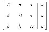
- The diagonal of the matrix is the set of elements that starts at the top, left corner and runs diagonally down and to the right. The diagonal of the above matrix consists of the numbers 4, 1 and 2.
- Any elements in position a are said to lie above the diagonal, and any in position
b are below the diagonal:
Keep in mind the following:
- the i-th row of the augmented matrix represents the i-th equation
- the j-th column (to the left of the vertical line) represents the (coefficients of the) j-th variable or unknown
- the vertical line represents the equal signs
Elementary Row Operations
Recall that an equation such as:7(x−4)=14,may be solved for x by applying the following operations:
- dividing both sides of the equation by the same value, namely 7, to yield x−4=2,
- then adding the same quantity to both sides, namely 4, to yield x=6.
Similarly, the solution of a system of equations is any set of values of all of the variables that satisfies all of the equations simultaneously. For example the system:
has the solution:
{x = 7, y = 5, z = 3}.
This can be verified by substituting these values into all three of the equations and producing three identities.
A system of equations can be solved by generalizing the two operations described above and observing that the solution of a system of equations is not changed by:
- dividing an both sides of an equation by a constant, or
- subtracting a multiple of one equation from another equation.
These same operations can be applied to the rows of an augmented matrix, since each row just represents an equation. They are then called Elementary Row Operations.
The Elementary Row Operations (E.R.O.'s) are:
- E.R.O.#1: Choose a row of the augmented matrix and divide (every element of) the row by a constant.
Example:
The notation means to divide the first row of the augmented matrix by 2 to produce the new augmented matrix.
- E.R.O.#2: Choose any row of the augmented matrix and subtract a multiple of any other row from it (element by element).
Example:
The notation means to take row 2 and subtract 3 times row 1 from it to produce the new augmented matrix.
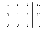
We will apply the E.R.O.'s in a certain sequence (the Gaussian elimination method, described below) to transform the augmented matrix into triangular echelon form. In this form the augmented matrix has 1's on the diagonal, 0's below the diagonal and any numbers above the diagonal. For example, the augmented matrix:
transformed into the triangular echelon form is:
This new augmented matrix represents the system of equations:
It is solved by back-substitution. Substituting z = 3 from the third equation into the second equation gives y = 5, and substituting z = 3 and y = 5 into the first equation gives x = 7. Thus the complete solution is:
{x = 7, y = 5, z = 3}.
Gaussian Elimination
In the Gaussian Elimination Method, Elementary Row Operations (E.R.O.'s) are applied in a specific order to transform an augmented matrix into triangular echelon form as efficiently as possible.
This is the essence of the method: Given a system of m equations in n variables or unknowns, pick the first equation and subtract suitable multiples of it from the remaining m-1 equations. In each case choose the multiple so that the subtraction cancels or eliminates the same variable, say x1. The result is that the remaining m-1 equations contain only n-1 unknowns (x1 no longer appears).
Now set aside the first equation and repeat the above process with the remaining m-1 equations in n-1 unknowns.
Continue repeating the process. Each cycle reduces the number of variables and the number of equations. The process stops when either:
- There remains one equation in one variable. In that case, there is a unique solution and back-substitution is used to find the values of the other variables.
- There remain variables but no equations. In that case there is no unique solution.
- There remain equations but no variables (ie. the lowest row(s) of the augmented matrix contain only zeros on the left side of the vertical line). This indicates that either the system of equations is inconsistent or redundant. In the case of inconsistency the information contained in the equations is contradictory. In the case of redundancy, there may still be a unique solution and back-substitution can be used to find the values of the other variables.
Examples of all these possibilities are given below.
Algorithm for Gaussian Elimination:
Transform the columns of the augmented matrix, one at a time, into triangular echelon form. The column presently being transformed is called the pivot column. Proceed from left to right, letting the pivot column be the first column, then the second column, etc. and finally the last column before the vertical line. For each pivot column, do the following two steps before moving on to the next pivot column:
- Locate the diagonal element in the pivot column. This element is called the pivot.
The row containing the pivot is called the pivot row. Divide every element in the pivot
row by the pivot (ie. use E.R.O. #1) to get a new pivot row with a 1 in the pivot position.
- Get a 0 in each position below the pivot position by subtracting a suitable multiple of the pivot row from each of the rows below it (ie. by using E.R.O. #2).
Upon completion of this procedure the augmented matrix will be in triangular echelon form and may be solved by back-substitution.
Example: Use Gaussian elimination to solve the system of equations:
Solution: Perform this sequence of E.R.O.'s on the augmented matrix. Set the pivot column to column 1. Get a 1 in the diagonal position (underlined):
Next, get 0's below the pivot (underlined):
Now, let pivot column = second column. First, get a 1 in the diagonal position:
Next, get a 0 in the position below the pivot:
Now, let pivot column = third column. Get a 1 in the diagonal position:
This matrix, which is now in triangular echelon form, represents:
It is solved by back-substitution. Substituting z = 3 from the third equation into the second equation gives y = 5, and substituting z = 3 and y = 5 into the first equation gives x = 7. Thus the complete solution is:
{x = 7, y = 5, z = 3}.
Example of Gaussian Elimination Applied to a Redundant System of Linear Equations
Use Gaussian elimination to put this system of equations into triangular echelon form and solve it if possible:
Solution: Perform this sequence of E.R.O.'s on the augmented matrix. Set the pivot column to column 1. There is already a 1 in the pivot position, so proceed to get 0's below the pivot:
Now, set the pivot column to the second column. First, get a 1 in the diagonal position:
Next, get a 0 in the position below the pivot:
Now, set the pivot column to the third column. The first thing to do is to get a 1 in the diagonal position, but there is no way to do this. In fact this matrix is already in triangular echelon form and represents:
This system of equations can't be solved by back-substitution because we have no value for z. The last equation merely states that 0=0. There is no unique solution because z can take on any value.
In general, one or more rows of zeros at the bottom of an augmented matrix that has been put into triangular echelon form indicates a redundant system of equations.
Example of Gaussian Elimination Applied to an Inconsistent System of Linear Equations
Use Gaussian elimination to put this system of equations into triangular echelon form and solve it if possible:
Solution: Perform this sequence of E.R.O.'s on the augmented matrix. Set the pivot column to column 1. There is already a 1 in the pivot position, so proceed to get 0's below the pivot:
Now, set the pivot column to the second column. There is already a 1 in the pivot position, so proceed to get 0's below the pivot:
Now, set the pivot column to the third column. The first thing to do is to get a 1 in the diagonal position, but there is no way to do this. In fact this matrix is already in triangular echelon form and represents:
This system of equations is inconsistent and has no solution. The last equation states a contradiction, namely 0 = −50.
In general, an augmented matrix which has been put into triangular echelon form and which contains one or more bottom rows consisting of all zeros to the left of the vertical line and a non-zero number to the right indicates an inconsistent system of equations with no solution.
