MathOnWeb.com

What it teaches:

This app teaches the Gauss-Jordan elimination method of solving a system of linear equations. Here is a screen shot:

Because the app allows only elementary row operations and because it does the arithmetic, you can stay focused on the method and not get bogged down by the details.

How it works:

• You start with either a new system of 2, 3, or 4 equations, or you can open a previously saved system of equations.
  
  
• Once all the coefficients are entered, you can either click on Automatic to go straight to the solution, or on Manual to solve the system yourself, step-by-step, by applying the three types of elementary row operations.
  
  
• In Manual mode you can click on Assist if you are stuck and the app will do the next step for you.
  
  
• As the screen shot shows, you first test a row operation. The tentative result is shown in red below the row that will change. If this is what you intended then the operation is carried out. (The idea is that you can see the system of equations both before and after the operation.)

Some ideas for teachers:

• You can start with a solution and reverse the Gauss-Jordan procedure; thus creating a question in which your students will encounter only integers when they solve it.
  
  
• By letting the right side of a system of equations be (1, 0, 0), then (0, 1, 0), then
  (0, 0, 1), you can explain the idea behind the inverse matrix.
  
  

What it teaches:

• This app teaches you how to design a planar (2 dimensional) truss,
  
  
• It teaches you how, by counting equations and unknowns, you can assess the stability of a truss (for example a triangle is stable but a rectangle is not),
  
  
• It shows how the assumption that the forces are in balance at every joint gives rise to a system of equations,
  
  
• It shows how the system of equations can be solved to give the tension or compression in each member of the truss and the force on each support of the truss.

How it works: There are three steps:

• Step 1: You design the truss. You select the Member tool (the leftmost tool on the toolbar) and then click and drag the mouse in the drawing area to create a truss member with a joint at either end. You repeat to add more members. (There are features such as snap to grid and snap to object to ensure that the members connect end-to-end at the joints.) You add forces (using the second tool) to load down your truss and you add supports (using the third and fourth tools) to hold up your truss. Here is a screen shot of a Parker truss:
  
  
  
  
  
  
• Step 2: You number the joints and give names to the forces in the truss members and the forces on the supports. This can be sped up by just letting the app choose the names by clicking on AutoName.
  
  
  
  
  
  
• Step 3: You let the app analyse the truss and you view the reports.
  
  To do the analysis the app assumes that:
  
  
  • Every member of the truss is under some unknown compression and is therefore providing a force toward the joint at either of its ends. This is indicated by the red arrows on all of the members. (If it turns out that some member is in fact under tension, this will result in a negative answer for that force.)
    
    
  • The truss is in equilibrium (standing still). This means that at every joint two equations hold: the forces right = the forces left, and the forces up = the forces down. For this example there are 9 joints x 2 equations / joint = 18 equations.
    
    
  The app gives several reports:
  
  
  • The number of equations and number of unknowns, and the implications for the stability of the truss. For this truss there are 18 equations and 18 unknowns, so a unique solution and hence stability is possible.
    
    
  • A listing of the system of equations for the entire truss. Also, by clicking on a joint, you can see the pair of equations that hold at that joint. The screen shot below shows an example.
    
    
  • A listing of the system of equations for the entire truss reduced to RREF (reduced row echelon form) thus giving the solutions of the equations.
  
  

Here is a screen shot showing the equations that are displayed if you click on joint 9 or joint 7 (the forces right = the forces left, and the forces up = the forces down).

Here is a screen shot of all of the equations assembled into an augmented matrix.

Here is a listing of the forces (the solution of the system of equations). The load that was placed at the middle of the span was 1000. Notice that:

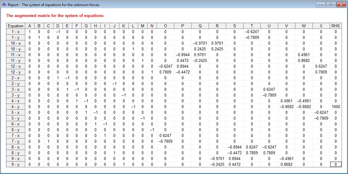
• B and C each support half of this load (500).
  
  
• A is zero because the load was applied straight down.
  
  
• Forces R, S, and T are all positive indicating that members near the top of the truss are under compression and forces D, E, and F are all negative indicating that members near the bottom of the truss are under tension.
  
  
• The biggest forces are Q and R at the very top of the truss so we should make those members extra strong.

Some ideas for teachers:

• The app comes with a helpfile that explains statics and truss analysis.
  
  
• The app comes with sample trusses files that result in overdetermined, inconsistent and redundant systems of equations.
  
  
• Start by building some very simple ‘trusses’ such as one having just one roller support, one member, and one force attached to it. You will get an inconsistent system of equations, which means that the assumption of equilibrium is invalid, so the truss will collapse.
  
  
• This is a great application of trigonometry.
  
  

What it teaches: This app teaches the nodal analysis method of solving DC electric networks. The basic idea is that applying Kirchhoff's Current Law at the various nodes of the network yields a system of equations whose simultaneous solution is the values of the node voltages. Here is a screen shot:

How it works: You draw an electric circuit by selecting various tools on the toolbar and then clicking or dragging in the main drawing area in the middle of the screen. Depending on the active button you can draw a piece of wire, a resistor, a current source, etc., or add, move, delete, change the value, direction, etc. of it.

When the circuit is complete, the app displays the nodes as red dots (and the supernodes as red lines) and you name the node voltages, which are the unknowns in the nodal analysis method. You may give some node voltage the name 0 (zero) and it then becomes the reference node.

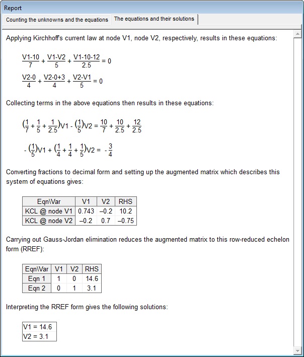
The app then displays the system of equations and their solution. Here is a screen shot:

Some ideas for teachers:

• If you teach math, this application provides a good example of how systems of equations arise in electrical engineering.
  
  
• If you teach electricity, then you can quickly show the effect of changing directions or values of elements and of changing the reference node.
  
  
• You can show how the number of unknowns and the number of equations is affected by using or not using a reference node, and by the presence of supernodes.
  
  
• You can set up homework and exam problems.
  
  

What it teaches: This app teaches the loop analysis method of solving DC electric networks. The basic idea is that an electric network can be considered to be a set of loops with a current flowing around each loop.  Applying Kirchhoff's Voltage Law around the various loops yields a system of equations whose simultaneous solution is the values of the loop currents. Here is a screen shot:

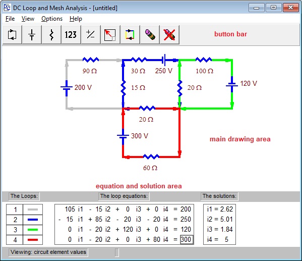
How it works: You draw an electric network by activating various tools on the button bar and then clicking or dragging in the main drawing area in the middle of the screen. Depending on the active button you can draw a loop, resistor, etc., or add, move, delete, change the value, direction, etc. of any element at any time.

As the network takes shape the system of equations for the loop currents and their solutions are immediately updated in the equation and solution area at the bottom of the screen.

If you click on a coefficient in the system of equations the part of the circuit responsible for that coefficient blinks. You can also change the display to show the currents through elements, the voltages across the elements or the power generated or consumed by the elements. When you are finished you can print a report on the circuit.

Some ideas for teachers:

• If you teach math, this application provides a good example of how systems of equations are used in electrical engineering.
  
  
• If you teach electricity, then you can quickly show the effect of changing loops, directions, elements, etc.
  
  
• You can illustrate the concepts of loops and meshes, series and parallel circuits, maximum power transfer, etc.
  
  
• You can set up homework and exam problems.
  
  

What it teaches: This program teaches the loop analysis method of solving AC electric networks. It is very similar to the DC Loop Analysis app except that it uses complex numbers to describe the impedance of inductors, resistors and capacitors; complex numbers in polar form (phasors) to describe voltages and currents; and complex arithmetic to solve the system of equations.

The basic idea of the loop analysis method is that an electric network can be considered to be a set of loops with a current flowing around each loop.  Applying Kirchhoff's Voltage Law around the various loops yields a system of equations whose simultaneous solution is the values of the loop currents. Here is a screen shot:

How it works: You draw an electric network by activating various tools on the button bar and then clicking or dragging in the main drawing area in the middle of the screen. Depending on the active button you can draw a loop, generator, inductor, etc., or add, move, delete, change the value, direction, etc. of any element at any time.

As the network takes shape the system of equations for the loop currents and their solutions are immediately updated in the equation and solution area at the bottom of the screen.

If you click on a coefficient in the system of equations the part of the circuit responsible for that coefficient blinks. You can also change the display to show the currents through elements, the voltages across the elements or the power dissipated by the elements. When you are finished you can print a report on the circuit.

Some ideas for teachers:

• If you teach math, this application provides a good example of how complex numbers are used in electrical engineering.
  
  
• If you teach electricity, you can quickly show the effect of changing loops, directions, elements, etc.
  
  
• You can illustrate the concepts of loops and meshes, series and parallel circuits, maximum power transfer, etc.
  
  
• You can set up homework and exam problems.
  
  

What it teaches:

The Simplex Wizard app teaches the Simplex Method of solving linear programming problems. It shows (1) how to set up the initial tableau for the problem and (2) how to solve the problem using Gaussian elimination. The wizard allows you to focus on the method and not get bogged down by the arithmetic. At every point in the procedure the status bar at the bottom of the wizard offers context-sensitive help on what to do next.

How it works: 

We will demonstrate with this linear programming problem: minimize the cost,

subject to the constraints:

Step 1.  Set up the initial tableau. The wizard asks you some general questions such as whether the objective is to maximize or minimize, how many variables appear in the constraints and how many and of what type are the constraints:

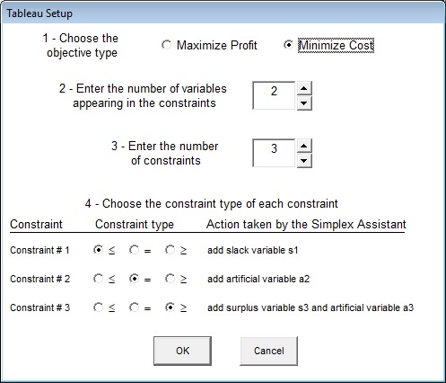
This is enough information for the wizard to create a tableau of the right size and to partially fill it in:

You finish setting up the tableau by filling in the names of the variables and the coefficients that appear in the constraints and objective function.

Now you can hover the mouse over each of the grids that make up the tableau and the status bar shows how to interpret the contents of that grid.

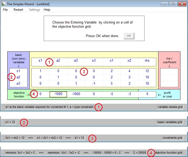
Step 2.  Apply the Simplex Method.  You choose an entering variable (column), you choose a leaving variable (row), the wizard does Gaussian elimination. These three operations are repeated until the solution is found. The status bar display helps you choose.

Here is the display at the point where you have to choose an entering variable. Notice that the wizard says “choose x1”.

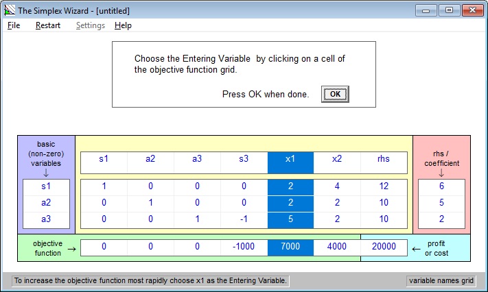
Now you have to pick an leaving variable (row). Notice that the wizard says “choose a3”.

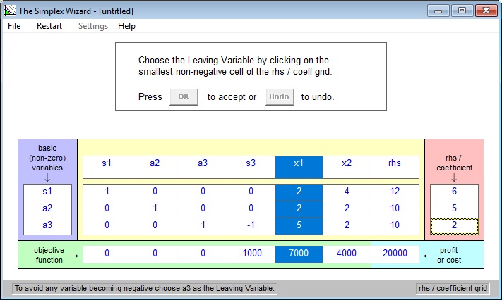
Now the wizard does Gaussian elimination on the tableau using the element at the intersection of the entering column and leaving row as pivot.

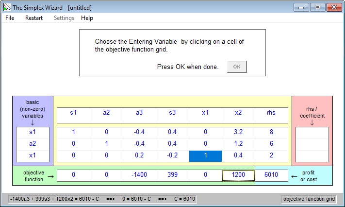
This process – choosing an entering column, a leaving row, Gaussian elimination – is repeated until the objective function is optimized as shown here:

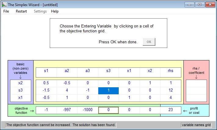
This final tableau says that the solution to our problem is a minimum cost of C = 23 and that this happens when x1 = 4 and x2 = 1.

Some other features of the Simplex Wizard are that you can save this simplex problem to a file, you can specify the number of significant figures to be displayed and you can print a report showing the steps that were used to solve the problem.

Some ideas for teachers:

• This application provides a good example of how systems of equations arise in economics.
  
  
• Using this app you can create more realistic problems that have more than just two or three constraints.
  
  

What it teaches:  This app describes visually the processes of differentiation, indefinite integration and definite integration (the area under the curve).

How it works:

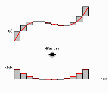
Visual Differentiation: You can draw a freehand curve or choose from a number of predefined curves. This curve is then digitized (broken into 10 or 15 straight line segments). When you click on differentiate the segments fall one-by-one onto the x axis and produce the derivative. Here is an example of the display after the animation is finished.

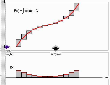
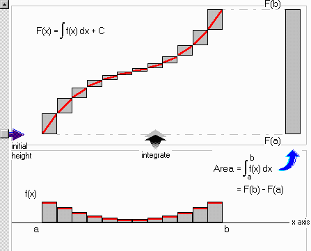
Indefinite Integration: You can draw a freehand curve or choose from a number of predefined curves. This curve is then digitized (broken into a number of rectangles). When  you click on integrate the segments rise one-by-one and arrange themselves end-to-end (i.e. integrate themselves) to produce the indefinite integral. Here is an example of the display after the animation is finished. Notice the movable pointer which represents where the indefinite integral starts.

Definite Integration or Area Under the Curve: This is exactly the same as the indefinite integration animation except that it continues with another animation in which the pieces of the integrated function move to the right to form a stack whose height represents the area under the original curve. Here is an example of the display part way through the animation:

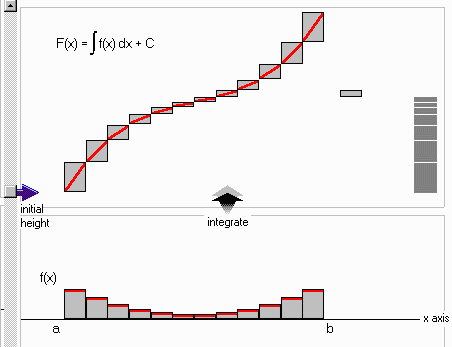
... and after the animation is finished:

Some ideas for teachers:

• In a regular calculus class students learn quite quickly that, for example, the integral of x² is ⅓x³+C, but they have problems understanding how to obtain the integral of a piecewise-defined function. What this app makes clear is that you don't have to integrate a formula; you can integrate any curve that you can sketch freehand.  The method is always the same – you join the pieces end-to-end.
  
  

What is it: A calculator that operates on complex numbers. There are actually two versions: the basic calculator and the stack calculator.

How it works:

The basic calculator. You type in two complex numbers, x and y, in either rectangular or polar coordinates. Then you click on an operation (addition, subtraction, multiplication, division, exponentiation or reciprocal) to produce a third complex number z. The calculator displays all three numbers in both polar and rectangular coordinates.

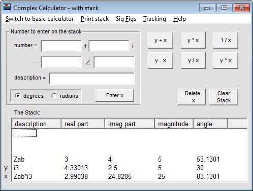
The stack calculator maintains a stack of complex numbers. When you type a complex number into the calculator it is put at the end (bottom) of the stack. When you do an operation, it is done on the last two complex numbers on the stack (called x and y), and the result is also put on the stack. The great thing about the stack is that chain calculations are easy to do because you can recall any of the numbers that are already on the stack.

Another feature is that each complex number that you enter can be given a text description. When you carry out an operation the result is automatically given a text description as well, based on the operands and the operation. In the example below we entered two numbers with the descriptions ‘Zab’ and ‘i3’. When we multiplied them the result was given the description ‘Zab*i3’. Another feature is that the contents of the stack can be pasted into a word processor.

What it teaches: This interactive tutorial teaches addition and subtraction of 2-dimensional vectors, resolution into x and y components, representation in polar and rectangular coordinates, and conversion between these coordinate systems.  Here is a screen shot of the contents:

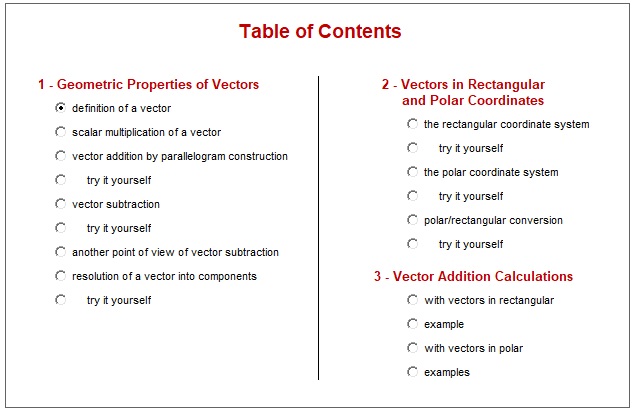
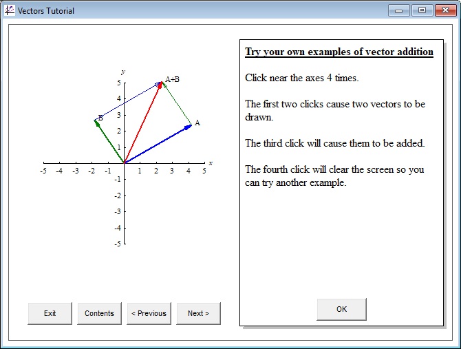
How it works: By double-clicking on a topic you jump to the screen associated with that topic. In each screen there is text on the right side explaining some concept and graphics on the left illustrating the concept. Most topics have a ‘try it yourself ’ section where you can create your own examples. Here is a screen shot:

What it teaches: This interactive tutorial teaches the concept of a rotating vector and how it generates a sinusoidal waveform. It uses animation to illustrate a topic that is very difficult to illustrate on a written page. Here is a screen shot of the contents:

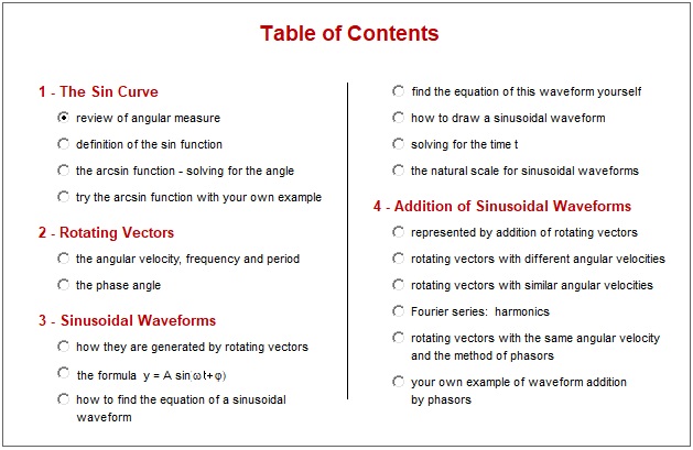
The purpose of part 1 is to make you familiar with the sine curve. When you are finished you will know how to solve an equation of the form

for all values of t, given the parameters A, ω and φ.

Then in part 2, via animation, you are introduced to rotating vectors and the concepts of angular velocity and phase angle.

In part 3 you see how waveforms correspond to rotating vectors.

In part 4 you see animations of various cases of the addition of sinusoidal waves, including Fourier series.

How it works: By double-clicking on a topic in the table of contents you jump to the screen associated with that topic. In each screen there is text on the right side explaining some concept and graphics on the left illustrating the concept. Most topics have a ‘try it yourself ’ section where you can create your own examples.

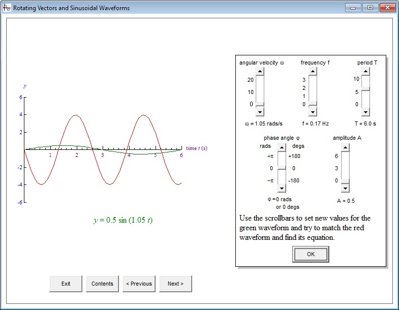
Here is a screen shot from the topic Sinusoidal waveforms - find the equation of this waveform yourself. By using the scroll bars you can adjust the values of the parameters ω, f, T, φ and A of the green waveform and try to make it identical to the (randomly generated) red waveform. This will help you understand the role of each of the parameters.

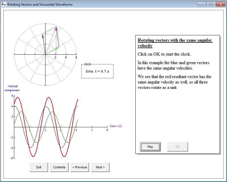
Here is a screen shot from the topic Addition of sinusoidal waveforms - rotating vectors with the same angular velocity. This topic illustrates the method of phasor addition (which is that you can add waveforms indirectly by adding the rotating vectors that generate them).