Simulated Annealing and the Travelling Salesman Problem


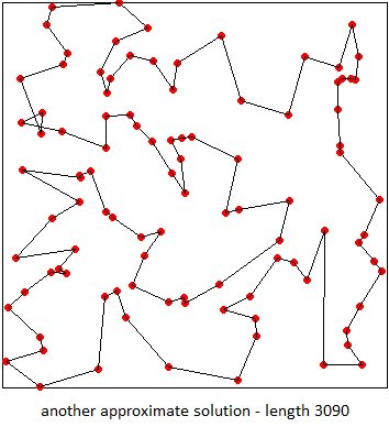
Figure 1. This animation shows 100 cities in a 350x350 area. A typical random path has a length of about 20,000. The shortest path may never be found. Two close-to-shortest paths found by simulated annealing both have a length of about 3000. On my computer they each take less than a second to find.
Given a list of cities and the distances between each pair of cities, the Travelling Salesman Problem (TSP) is to find the shortest path that visits each city exactly once and returns to the home city.
We showed how exhaustive search finds the exact solution for this problem in another blog page. Unfortunately that takes an impractically long time for more than, say, 12 cities. (For example for 20 cities my computer would take 2 million years!)
Here we present another method, call simulated annealing, that finds an approximate solution very quickly (for 100 cities my computer takes less than a second).
You can download an Excel spreadsheet with the code here.
Simulated annealing is based on an analogy with thermodynamics, specifically what is happening at the atomic level when a liquid freezes and crystallizes. At high temperatures, the atoms of the liquid move freely. If the liquid is cooled, the atoms lose their mobility. As the liquid freezes the atoms line themselves up and form a crystal lattice. The rate of cooling is critical. If the system is cooled rapidly (quenched) then the resulting crystal lattice is full of defects. This is a state of high potential energy. If it is cooled slowly enough (annealed) then the result can be a perfect crystal, free of defects. This is the state of minimum potential energy for the lattice.
Simulated annealing makes three analogies. (1) The potential energy of the crystal lattice is analogous to the path length in the Travelling Salesman Problem. (2) Temperature is analogous to accepting longer paths as we wander from path to path in our search to find the shortest path. (3) Annealing (slow cooling) is analogous to slowly eliminating the longer paths from our search.
Contents of this page
- Combinatorial Minimization
- Potential Energy of a Crystal
- Temperature of a System
- Simulated Annealing Algorithm
- Simulated Annealing Spreadsheet and Code
- Conclusions
Combinatorial Minimization
Definition: Minimization is the process of finding the global minimum of a function. Combinatorial minimization is the process of searching for the minimum of a function whose domain is a discrete but large configuration space (as opposed to a continuous space).

Figure 2. In continuous minimization the domain, x, of the function is continuous. We can use derivatives to find the global minimum, G.
If you have studied calculus then you are familiar with continuous minimization, where the domain, x, of the function is continuous (i.e. the x axis has no gaps).
Consider, for example, the function in Fig. 2. If the function is smooth enough then we can find the global minimum, G, by first finding all the locations where the derivative is zero (this includes L and G) and then dropping L because G is smaller.
We can also use numerical analysis and try to find G by starting at an arbitrary point like B and using the derivative to go downhill. The problem is that if we start at the wrong point, A, then going downhill leads us to the local minimum, L. To prevent this we must know something about our function; for example, does it have one local minimum or many.

Figure 3. In the Travelling Salesman Problem the domain is a large number of discrete points, namely all the possible paths. This type of domain is called a configuration space and finding the minimum is called combinatorial minimization.
Unfortunately, these concepts (continuous domain, smooth function, derivative) do not exist for the Travelling Salesman Problem. Instead we have the picture shown in Fig. 3, where the domain is a very large number of discrete points, each point representing a possible path. This type of domain is called a configuration space. In another blog page we learned how to count the paths (for example, for 4 cities there are 4! paths) and we learned how to list them (1234, 1243, etc). The paths can be arranged on the x axis in many ways, and closeness or going left or right on the x axis doesn't mean anything. Finding the minimum of this type of function is called combinatorial minimization.
Keep in mind that the configuration space for say, 100 cities, is vastly larger than the number of particles in the visible universe so we cannot hope to find the global minimum, or even recognize it if we did.
Potential Energy of a Crystal
As mentioned in the introduction, simulated annealing is based on three analogies. In this section we look at how the potential energy of the crystal lattice is analogous to the path length in the Travelling Salesman Problem.

Figure 4. The van der Waals force between two atoms is (a) repulsive at short distances, and (b) attractive at long distances.
Fig. 4(a) shows two identical atoms. Each atom has a positively clarged nucleus and a negatively charged electron cloud. They feel a Coulomb force that is strongly repulsive at short distances (a). But due to fluctuations in the electron clouds they feel a weak attractive force at long distances (b). This distance-dependent force is called the van der Waals force.

Figure 5. Potential energy diagram for the van der Waals force. Imagine a marble (or roller coaster) rolling down the red curve. It will oscillate between two points like b and c, before losing its energy and coming to a stop at a.
It is convenient to describe the van der Waals force in terms of its potential energy diagram. This is shown in Fig. 5. (If you have read the roller coaster blog page then you know that the roller coaster's profile is essentially a potential energy diagram.)
Understanding the potential energy diagram
- Fig. 5 shows the potential energy V of two atoms as a function of the distance r between the centers of the atoms.
- The force F between the two atoms is the negative gradient of the potential energy. That is, F = −dV/dr. Thus they feel a force pulling them together if r > a and a force pushing them apart if r < a.
- Point a is described as the bottom of the "potential well". As we will see in the next section on temperature, this is the spacing of two atoms in equilibrium at 0 K (absolute zero temperature). (Note that in this blog page we use the Kelvin temperature scale.)
- If we warm the two atoms up, they will gain the energy to climb higher and higher up the potential well. They will vibrate between points like b and c.
- Midway between b and c is d, and as we go higher and higher in the potential well, d moves to the right, following the dashed line. This explains why metals expand as they are heated.
- If the two atoms are heated enough, they have enough energy to climb out of the potential well and go their own ways (the spacing r → ∞). This explains melting.

Figure 6. Crystal lattice with different types of defects: (a) line defect, (b) interstitial atom, (c) vacancy.
Question: Suppose that we have a large number of atoms, not just two. What arrangement of atoms will produce the minimum potential energy?
Answer: A "perfect" crystal lattice with spacing a between nearest neighbor atoms.
One complication is that the lattice will invariably contain defects, like those shown in Fig. 6. Each defect results in an interatomic spacing that is not the ideal, a, and thus raises the potential energy of the crystal.
Here is an analogy: Picture thousands of soldiers standing around on a parade field. They are given the order to come to attention as quickly as possible. If they are given no guidance about where to start or which direction to face, then the resulting ranks would look similar to Fig. 6.
Conclusions:
- The perfect crystal has the lowest potential energy.
- Each defect raises the potential energy.
- The possible crystal lattices form a configuration space.
- The potential energy of the crystal lattice is analogous to the path length in the Travelling Salesman Problem.
Crystallography is a huge and fascinating field. You can get much more information at chem.libretexts.org, including types of crystal structures, types of defects and much more.
Temperature of a System
Now let's look at the second analogy that simulated annealing is based on: temperature is analogous to accepting longer paths, as we move among the possible paths in our search for the shortest path. To understand this analogy we must answer the question: “what exactly is temperature?”
James Clerk Maxwell and Ludwig Boltzmann pioneered the field that is now called statistical mechanics. (This is the field in which I got my Ph.D.) Their aim was to apply statistics to the motions of atoms. They wanted to understand the origin of temperature, pressure, etc., in the simplest possible system: an ideal gas. This is a gas whose particles move freely except for rare collisions in which they exchange energy and momentum with each other.
They discovered that when the gas is in|
| (1) |
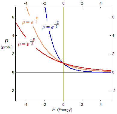
Figure 7. The Boltzmann distribution, eq. (1), as a function of energy for three temperatures. The red curve is the distribution at a high temperature; blue is at low temperature.
In this formula ∝ means "is proportional to", T is the temperature in kelvin and k is a constant called the Boltzmann constant.
Fig. 7 shows the Boltzmann distribution as a function of energy for three different temperatures: cold (blue), warm (orange), hot (red).
Note the following:
- At any given temperature low energy particles are more plentiful than high energy particles.
- If we raise the temperature, the distribution shifts to favor the high energy particles.
- There is always a non-zero probability that a particle will have an energy that is arbitrarily high.
The Boltzmann Distribution applied to an Ideal Gas
- The energy of an ideal gas is entirely due to the kinetic energy of the particles. For each particle it is given by the formula ½mv2, where m is the mass of the particle and v is its velocity.
- Velocity is a vector with components vx, vy, vz. The speed is the magnitude of the velocity.
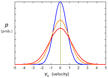
- Thus we can also graph the distribution of particles as a function of, say, the x component of the velocity (left), and as a function of speed (right):
 |
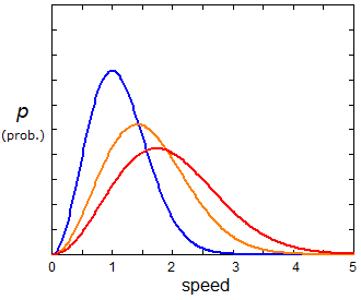 |
Figure 8. The Boltzmann distribution, (left) as a function of the x component of the velocity, and (right) as a function of the speed. As in Fig. 7 the red curves are at high temperature, the blue curves are at low temperature.
- Note that Figs. 7 and 8 are not contradictory! Fig. 7 says that low energies are more probable than high energies. Fig. 8(left) says that half the particles are moving to the left and half to the right. Fig. 8(right) says there is a most probable speed. (Note that a speed of zero is extremely unlikely because it requires that vx, vy, vz are all zero.)
- Calculus can be used to show that the peak of the speed graph occurs when v = (2kT/m)½ or when ½mv2 = kT. Thus the quantity kT is a measure of the kinetic energy of the particles in the gas. Boltzmann's constant, k, is one of the defining constants in physics.
- The most probable speed is very close to the speed of sound in the gas. Note that it increases with temperature.
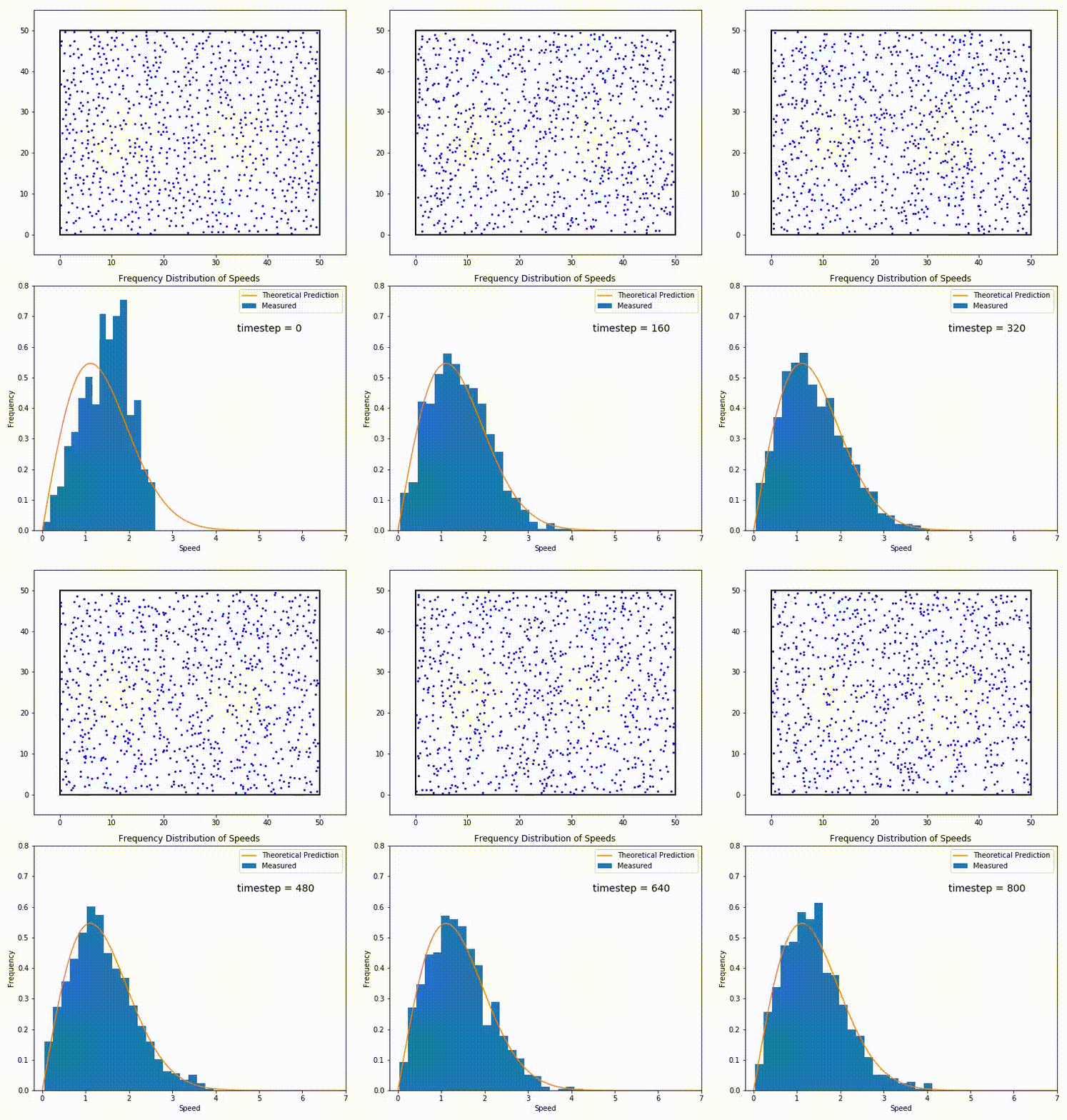
Figure 9. (top) Simulation of an ideal gas.
(bottom) Histogram of observed speeds. The orange curve is the speed distribution of Fig. 8.
Credit: By Dswartz4 - Own work, CC BY-SA 4.0
- The animation in Fig. 9 shows a simulation of a gas relaxing toward
thermodynamic equilibrium.
(The gas starts slightly out-of-equilibrium at timestep 0.)
- The graph in Fig. 9 is a histogram of the speeds seen in the simulation (how frequently each speed occurs). The histogram is superimposed on the speed distribution. Notice the excellent agreement.
- Note: If a system does not obey the Boltzmann distribution then it does not have a well-defined temperature. One example is a particle beam where all the particles have the same velocity.
The Boltzmann distribution applies not just to ideal gases, but to systems in general. If a system can be in different energy states and is in thermodynamic equilibrium, then the probability that the system is in any energy state is given by the Boltzmann distribution.
Simulated Annealing Algorithm

Figure 10. The simulated annealing algorithm starts with some path and applies a random permutation to it to generate another path. If this path satisfies the Metropolis criterion then it becomes the new path and process is repeated. There are two nested loops. The outer loop is used to lower the temperature in the Metropolis criterion.
Here is the algorithm in flowchart form and point form:
- We start with a list of the cities to visit (in no particular order). We calculate the the length of the path if they are visited in the order listed. We set the initial "temperature", T, to "high" (explained later).
- We make a tentative permutation of the list (a change to the order of the cities) and calculate how that would change the length of the path (call it ΔLength). The permutation is random.
- We apply the Metropolis function to the proposed length change. This is a
Boolean
function; i.e. it returns only two values: True (a.k.a. Yes or 1)
and False (a.k.a. No or 0).
The function works like this: If the path is shorter, then it always returns True. If the path is longer, then it may return True, with high probability at high temperature and with low probability at low temperature. - If the Metropolis function does return True then the proposed path becomes the new path. Otherwise, not.
- We go to step 2 and repeat.
- At intervals we lower the temperature, thus making the Metropolis function less likely to return True for longer paths. The two loops are nested so we do many permutations at many temperatures.
- Eventually we can't find any shorter path, so we accept the current path as the shortest path.
Details of the permutations in step 2
We must be able to wander freely in configuration space and create any possible path. This can be done by applying two basic permutations repeatedly: either reversing a segment of the path or moving the segment elsewhere. Here is an example of each:

We use a random number generator to
- choose a segment at random,
- choose the type of permutation (reverse or move) at random,
- and if it is a move, choose the destination at random.
Details of the Metropolis function in step 3
A permutation can either decrease or increase the path length. If we only accepted permutations that decreased the path length then we would risk falling into a local minimum, getting trapped, and being unable to get to the global minimum. We can avoid this if we also accept permutations that increase the path length, thus enabling us to get back out.
If we accept large increases in path length at first, then we will wander more-or-less freely in configuration space, and if we slowly reduce those acceptable increases, then there is a higher likelihood of falling into the global minimum.
To start let the "temperature", T, be merely a number that describes the largest path length increase that we will accept. (That is, when T is high we will accept large length increases, and when T is low we will only accept small length increases.) Here is a picture of a Boolean function that returns True if the change in path length, ΔLength, is less than T, and False otherwise:

and here is the Visual Basic code for it:
Function Foo(DLength As Single, T As Single) As Boolean
  'DLength, the change in path length, can be anything.
  'T, the temperature, must be positive or zero.

  If DLength < T then Foo = True
End Function
The problem with this function is that it is not the one used by nature. We saw above that a thermodynamic system obeys the Boltzmann distribution. Nicholas Metropolis came up with a better function based on the Boltzmann distribution. Here is a picture of it:
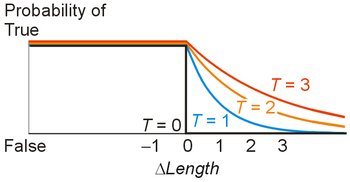
Note the following:
- The height of the curve is given by the formula

| (2) |
- The height of the curve is not the value returned by the Metropolis function. Rather, the height of the curve is the probability that the Metropolis function returns the value "True".
- There is a low but non-zero probability that a path will be accepted, no matter how much longer it is.
- If you are familiar with exponential decay then you will notice that T is analogous to a time constant.
Here is the code for Metropolis' function:
Function Metropolis(DLength As Single, T As Single) As Boolean   '1
  'Metropolis always returns True if DLength < 0,
  'and with probability exp(-DLength/T) if DLength > 0.
  'Rnd returns random numbers uniformly between 0 and 1.

  If DLength < 0 Then Metropolis = True: Exit Function           '2
  If Rnd < Exp(-DLength / T) Then Metropolis = True              '3
End Function                                                     '4
Note that the Rnd function in line 3 is a built-in function in Visual Basic that generates pseudo-random real numbers uniformly between 0 and 1.
Simulated Annealing Spreadsheet and Code
Here is the spreadsheet for the simulated annealing algorithm. The circled numbers refer to the notes below.

Notes on the spreadsheet:
Clicking the Set Up First button runs the subroutine SetUpMap (listed in the main code below). SetUpMap does the following six things:
- It reads in the number of cities and a seed number for the random number generator (in the first two yellow cells).
- It uses the seed to generate random locations for the cities. The cities' names are in column A, and their x and y coordinates are in B and C. (Each seed produces a different random map of cities.)
- This list is used by Excel to create a dot plot of the cities.
- It copies the list in columns A,B,C to columns J,K,L.
- The list in columns J,K,L is used by Excel to create a line plot. This is the initial path.
- It calculates the initial path length.
Clicking the TSP Anneal button then runs the main subroutine, called TSPAnneal (also listed in the main code below). It does two things:
- It reads in the rest of the values in the yellow cells: information about the temperature steps, another seed number (each seed produces a different but repeatable set of "random" permutations), and limits on the number of permutations to try.
- It runs through the two nested loops shown in the flowchart in Fig. 10. Each time the inner loop finishes (i.e. after every temperature drop) a message box pops up, the path list 4 and the path chart 5 are updated, and information on the progress 8 is shown. When no shorter path can be found, TSPAnneal quits. The spreadsheet then looks like this:

Here is the Visual Basic code for the simulated annealing algorithm. To use it, copy both the main and the auxiliary code into an Excel module. (Click here to go to the blog page explaining VB programming for Excel.) The code assumes that the spreadsheet is organized as shown above.
Option Explicit                                                                          '1
Private Cities As Integer, X() As Single, Y() As Single, Slot() As Integer               '2
'------------------------------------------------------------------------------------------
Public Sub SetUpMap()                                                                    '3
  'Read in the number of cities and the random seed for
  'the map and set up the spreadsheet's cells and charts.
  Const MapWidth = 350                                                                   '4
  Dim SeedCity As Integer, I As Integer, PathLength As Single                            '5

  Range("A13:C400").ClearContents                                                        '6
  Range("P2:Q7").Copy Destination:=Range("J2:K7")                                        '7
  Cities = Cells(1, 6)                          'Number of cities.                       '8
  SeedCity = Cells(2, 6)                        'Seed for random location of cities.     '9
  Call Rnd(-SeedCity)                           'Reset Rnd with - argument.              '10

  ReDim X(1 To Cities) As Single, Y(1 To Cities) As Single, Slot(1 To Cities) As Integer '11

  For I = 1 To Cities                                                                    '12
    X(I) = MapWidth * Rnd                       'Set X(I) and Y(I) coords of city #I.    '13
    Y(I) = 350 - MapWidth * Rnd                 'Set Slot. eg: Slot(5)=3 means           '14
    Slot(I) = I                                 '5th city visited is city #3.            '15

    Cells(12 + I, 1) = Slot(I)                  'Copy X(), Y(), Slot() to                '16
    Cells(12 + I, 2) = X(I)                     'columns A,B,C.                          '17
    Cells(12 + I, 3) = Y(I)                     'Used for the cities chart.              '18
  Next I                                                                                 '19

  Range("A13:C300").Copy Destination:=Range("J13:L300")    'Initialize the path chart.   '20
  Cells(Cities + 13, 10) = Cells(13, 10)                   'Close the path.              '21
  Cells(Cities + 13, 11) = Cells(13, 11)                                                 '22
  Cells(Cities + 13, 12) = Cells(13, 12)                                                 '23

  For I = 1 To Cities                           'Calculate the initial path length.      '24
    If I < Cities Then                                                                   '25
      PathLength = PathLength + Pyth(X(I), Y(I), X(I + 1), Y(I + 1))                     '26
    Else                                                                                 '27
      PathLength = PathLength + Pyth(X(I), Y(I), X(1), Y(1))                             '28
    End If                                                                               '29
  Next I                                                                                 '30

  Cells(3, 10) = PathLength                                                              '31
End Sub                                                                                  '32
'------------------------------------------------------------------------------------------
Public Sub TSPAnneal()                                                                   '33
  Dim Seg(1 To 6) As Integer                                                             '34
  Dim PathLength As Single, DLength As Single                                            '35
  Dim RandSeed As Integer, PermuType As Integer, NN As Integer                           '36
  Dim NTries As Long, PermutNum As Long, I As Long                                       '37

  Dim T As Single, TFactor As Single, TNum As Integer                                    '38
  Dim NLimit As Long, Nsucc As Long, J As Integer                                        '39
                                'Input:
  PathLength = Cells(3, 10)     'initial path length calculated in SetUpMap,             '40
  T = Cells(4, 6)               'the initial temperature,                                '41
  TNum = Cells(5, 6)            'number of temperatures to use,                          '42
  TFactor = Cells(6, 6)         'ratio of newT/oldT as T is lowered,                     '43
  RandSeed = Cells(7, 6)        'seed for random number generator,                       '44
  NTries = Cells(8, 6)          'number permutations to attempt at each temp,            '45
  NLimit = Cells(9, 6)          'limit on number of successful perms at each temp        '46

  Cells(3, 11) = T                                                                       '47
  Call Rnd(-RandSeed)           'Reset Rnd to specific start with - argument.            '48
  PermutNum = 0                 'Number of permutations actually made.                   '49

  For J = 1 To TNum             'OUTER LOOP: cycle through temperature steps             '50
    Cells(5, 10) = J                                                                     '51
    Cells(5, 11) = T                                                                     '52
    Nsucc = 0                                                                            '53

    For I = 1 To NTries         'INNER LOOP: cycle through permut. attempts              '54
10:   Seg(1) = 1 + Int(Cities * Rnd)                         'Choose beginning and       '55
      Seg(2) = 1 + Int((Cities - 1) * Rnd)                   'end of a segment.          '56
      If (Seg(2) >= Seg(1)) Then Seg(2) = Seg(2) + 1                                     '57
      NN = 1 + ((Seg(1) - Seg(2) + Cities - 1) Mod Cities)   'NN Cities not on segment.  '58
      If NN < 3 Then GoTo 10                                                             '59

      PermuType = Int(2 * Rnd)                          'Flip a coin                     '60

      If PermuType = 0 Then                             'If heads then try a move.       '61
        Seg(3) = Seg(2) + Int(Abs(NN - 2) * Rnd) + 1                                     '62
        Seg(3) = 1 + ((Seg(3) - 1) Mod Cities)          'Move to after Seg(3)            '63
        DLength = MoveCost(Seg)                         'Calculate DLength of move.      '64
      Else                                              'If tails then try reversal.     '65
        DLength = ReverseCost(Seg)                      'Calculate DLength of reversal.  '66
      End If                                                                             '67

      If Metropolis(DLength, T) Then                    'Carry out move/reversal.        '68
        If PermuType = 0 Then Call Move(Seg) Else Call Reverse(Seg)                      '69
        PermutNum = PermutNum + 1                                                        '70
        PathLength = PathLength + DLength                                                '71
        Nsucc = Nsucc + 1                                                                '72
      End If                                                                             '73

      If Nsucc >= NLimit Then Exit For                  'temperature is too high         '74
    Next I                                              'End of inner loop               '75

    Call Display(PermutNum, PathLength)                 'Comment this for Statistics     '76
    MsgBox "Temperature step"                           'Comment this for Statistics     '77
    T = T * TFactor                                                                      '78

    If Nsucc = 0 Then Exit For                          'temperature is too low          '79
  Next J                                                'End of outer loop               '80

  Call Display(PermutNum, PathLength)                   'Display end of simulation       '81
End Sub                                                                                  '82
'------------------------------------------------------------------------------------------
Private Function Metropolis(DLength As Single, T As Single) As Boolean                   '83
  'Returns True if DLength < 0 and with prob exp(-DLength/T) if DLength > 0

  If DLength < 0 Then Metropolis = True: Exit Function                                   '84
  If DLength >= 85 * T Then Metropolis = False: Exit Function     'Avoid overflow        '85
  If Rnd < Exp(-DLength / T) Then Metropolis = True                                      '86
End Function                                                                             '87
Private Function Pyth(X1 As Single, Y1 As Single, X2 As Single, Y2 As Single) As Single '88
'Pythagoras distance between points (X1, Y1) and (X2, Y2).
Pyth = Sqr((X2 - X1) ^ 2 + (Y2 - Y1) ^ 2) '89
End Function '90
'------------------------------------------------------------------------------------------
Private Function ReverseCost(Seg) As Single '91
'Return the change in path length if the segment defined by Seg is reversed
Dim J As Integer, II As Integer '92
Dim XX(1 To 4) As Single, YY(1 To 4) As Single '93
Seg(3) = 1 + (Seg(1) + Cities - 2) Mod Cities '94
Seg(4) = 1 + Seg(2) Mod Cities '95
For J = 1 To 4 '96
II = Slot(Seg(J)): XX(J) = X(II): YY(J) = Y(II) '97
Next J '98
ReverseCost = -Pyth(XX(1), YY(1), XX(3), YY(3)) _
- Pyth(XX(2), YY(2), XX(4), YY(4)) _
+ Pyth(XX(1), YY(1), XX(4), YY(4)) _
+ Pyth(XX(2), YY(2), XX(3), YY(3)) '99
End Function '100
'------------------------------------------------------------------------------------------
Private Function MoveCost(Seg) As Single '101
'Return the change in path length is the segment defined by Seg is moved
Dim J As Integer, II As Integer '102
Dim XX(1 To 6) As Single, YY(1 To 6) As Single '103
Seg(4) = 1 + Seg(3) Mod Cities '104
Seg(5) = 1 + (Seg(1) + Cities - 2) Mod Cities '105
Seg(6) = 1 + Seg(2) Mod Cities '106
For J = 1 To 6 '107
II = Slot(Seg(J)): XX(J) = X(II): YY(J) = Y(II) '108
Next J '109
MoveCost = -Pyth(XX(2), YY(2), XX(6), YY(6)) _
- Pyth(XX(1), YY(1), XX(5), YY(5)) _
- Pyth(XX(3), YY(3), XX(4), YY(4)) _
+ Pyth(XX(1), YY(1), XX(3), YY(3)) _
+ Pyth(XX(2), YY(2), XX(4), YY(4)) _
+ Pyth(XX(5), YY(5), XX(6), YY(6)) '110
End Function '111
'------------------------------------------------------------------------------------------
Private Sub Reverse(Seg) '112
'Reverse the segment in Seg
Dim NN As Integer, J As Integer, K As Integer, L As Integer, Itmp As Integer '113
NN = (1 + (Seg(2) - Seg(1) + Cities) Mod Cities) \ 2 '114
For J = 1 To NN '115
K = 1 + (Seg(1) + J - 2) Mod Cities '116
L = 1 + (Seg(2) - J + Cities) Mod Cities '117
Itmp = Slot(K) '118
Slot(K) = Slot(L) '119
Slot(L) = Itmp '120
Next J '121
End Sub '122
'------------------------------------------------------------------------------------------
Private Sub Move(Seg) '123
'Move the segment defined by Seg
Dim M1 As Integer, M2 As Integer, M3 As Integer '124
Dim NN As Integer, J As Integer, JJ As Integer '125
Dim Jorder() As Integer '126
ReDim Jorder(1 To Cities) '127
M1 = 1 + (Seg(2) - Seg(1) + Cities) Mod Cities '128
M2 = 1 + (Seg(5) - Seg(4) + Cities) Mod Cities '129
M3 = 1 + (Seg(3) - Seg(6) + Cities) Mod Cities '130
NN = 1 '131
For J = 1 To M1 '132
JJ = 1 + (J + Seg(1) - 2) Mod Cities '133
Jorder(NN) = Slot(JJ): NN = NN + 1 '134
Next J '135
For J = 1 To M2 '136
JJ = 1 + (J + Seg(4) - 2) Mod Cities '137
Jorder(NN) = Slot(JJ): NN = NN + 1 '138
Next J '139
For J = 1 To M3 '140
JJ = 1 + (J + Seg(6) - 2) Mod Cities '141
Jorder(NN) = Slot(JJ): NN = NN + 1 '142
Next J '143
For J = 1 To Cities '144
Slot(J) = Jorder(J) '145
Next J '146
End Sub '147
'------------------------------------------------------------------------------------------
Private Sub Display(PermutNum, PathLength As Single) '148
Dim I As Integer '149
For I = 1 To Cities 'Update table for the path chart. '150
Cells(12 + I, 10) = Slot(I) 'eg: Slot(5)=3 means 5th '151
Cells(12 + I, 11) = X(Slot(I)) 'city visited is city #3. '152
Cells(12 + I, 12) = Y(Slot(I)) '153
Next I '154
Cells(Cities + 13, 10) = Cells(13, 10) 'Close the path. '155
Cells(Cities + 13, 11) = Cells(13, 11) '156
Cells(Cities + 13, 12) = Cells(13, 12) '157
Cells(7, 10) = PermutNum 'Update permutation number '158
Cells(7, 11) = PathLength 'and path length '159
DoEvents 'DoEvents passes control to Windows '160
End Sub 'so path chart can be updated. '161
'------------------------------------------------------------------------------------------
Public Sub Statistics() '162
'Simulate quenching and annealing, each 200 times, using different seeds.
'Comment out lines 76 and 77 in Anneal to speed it up.
Dim I As Integer '163
'Simulate quenching:
Cells(4, 6) = 0: Cells(5, 6) = 1: Cells(8, 6) = 50000: Cells(9, 6) = 50000 '164
For I = 1 To 200 '165
Cells(7, 6) = I '166
Call SetUpMap '167
Call TSPAnneal '168
Cells(I + 28, 14) = Cells(7, 6) '169
Cells(I + 28, 15) = Cells(7, 10) '170
Cells(I + 28, 16) = Cells(7, 11) '171
Next I '172
'Simulate annealing:
Cells(4, 6) = 125: Cells(5, 6) = 50: Cells(8, 6) = 3000: Cells(9, 6) = 1500 '173
For I = 1 To 200 '174
Cells(7, 6) = I '175
Call SetUpMap '176
Call TSPAnneal '177
Cells(I + 28, 18) = Cells(7, 6) '178
Cells(I + 28, 19) = Cells(7, 10) '179
Cells(I + 28, 20) = Cells(7, 11) '180
Next I '181
MsgBox "Finished" '182
End Sub '183
Notes on the code:
- If you downloaded the spreadsheet then you can run the code by clicking on the Set up First button and then the TSP Anneal button on the Anneal sheet. You can get the statistics described in the Conclusions section below by clicking the Statistics button on the Statistics sheet.
- The code presented here is based on code in section 10.9 of Numerical Recipes by Press, Teukolsky, Vetterling and Flannery.
- The numbering scheme used here for the cities differs from that in the TSP blog page. Here, we are searching for the shortest loop connecting, say, 100 cities, and the home city is just one of the 100 cities. Once we have found the shortest loop then it is an easy matter to designate any city as the home city and go in either direction around the loop.
- The Rnd function
is a built-in function in Visual Basic that generates pseudo-random real numbers
between 0 and 1 (including 0, but excluding 1).
By using the formula
we can also use it to generate random integers in the range {lowerbound, ..., upperbound}. It is used in:Int((upperbound - lowerbound + 1) * Rnd) + lowerbound- lines 13 and 14 to generate random coordinates for the cities,
- lines 55 and 56 to pick a random segment of the path,
- line 60 to "toss a coin" (generate random 0's and 1's) to decide whether to move the segment or reverse the segment,
- line 62 to randomly choose where to move the segment.
- line 86 to randomly return True or False from the Metropolis function.
- Just as the hours on a clock run from 1 to 12 and then restart at 1, we want
to be able to go around the loop of cities. This can be done using the
Mod operator
which is just like the / (division) operator except that it returns the
remainder only. For example, if we enter the code
into the Immediate Window we get this printed:For I = 1 To 9: Print 1 + (I - 1) Mod 3,: Next I
The snippet1 2 3 1 2 3 1 2 31 + ··· Mod Citiesis used in many places in the code to loop around the cities.
Conclusions

The graph to the right shows the results of running the simulated annealing code 200 times and plotting the shortest path length found each time and the number of permutations required to get it. The runs differ only in the seed number used to initialize the random number generator.
Each run produced a different result. This implies that the configuration space has many local minima. Each point in the graph is one of them.
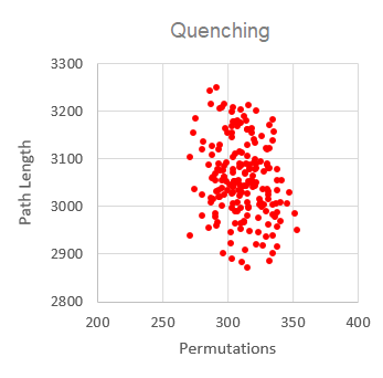
It is interesting to investigate whether simulated annealing (using the Metropolis criterion) is actually any better at finding the global minimum than quenching (simply going downhill). We can simulate quenching in the code by using just one temperature, and making that temperature zero. See line 164 in the subroutine Statistics.
The result of 200 quenching simulations is shown to the right. Notice that only an average 315 permutations were required to get these results. This is, of course, because longer-path permutations are not accepted.

Figure 11. Comparison of quenching and simulated annealing results. Statistically, simulated annealing is better at finding the shortest path.
If we only look at the shortest paths found, we get the histograms shown in Fig. 11. The shortest paths for simulated annealing were found to be normally distributed with a mean length of 2946 and a standard deviation of 56. The shortest paths for quenching were found have a mean length of 3017 and a standard deviation of 67.
Thus we can conclude that statistically, simulated annealing is better, at the cost of requiring more permutations.
If you would like to leave a comment or ask a question please send me an email!