Chapter 6 - Graphs, Linear Functions and Straight Lines

This chapter discusses graphs, linear functions and straight lines. It contains the following sections:

section 6.1 - In this section we introduce rectangular coordinates, graphs and how to locate points on a graph.
section 6.2 - In this section we talk about linear functions and their graphs, which are straight lines.
section 6.3 - In this section we talk about other types of graphs such as parametric graphs and contour graphs. We also explain how to solve equations graphically.

6.1 - Rectangular coordinates

The cartesian plane

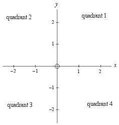A plane is a flat 2-dimensional region such as the surface of a page.

To specify locations on the plane we can lay down two number lines or axes perpendicularly on the plane as shown to the right. The horizontal axis is usually called the x axis and the vertical axis is usually called the y axis. The point where the axes cross is usually chosen to be where x = 0 and where y = 0 (this point is called the origin). The origin is indicated by a circle in the center of the picture. The axes divide the plane into four regions called quadrants, which are numbered counterclockwise as shown. This construction, a plane plus two perpendicular axes, is called a cartesian plane (named after René Decartes, 1596 - 1650).

If we draw points on a cartesian plane or if we draw a curve representing a function on a cartesian plane then we say that we are graphing or drawing a graph of the points or of the function.

The study of geometric shapes such as lines, circles, triangles, etc. can be done on the ordinary, blank plane or on the cartesian plane. When done on the ordinary plane, their study is called plane geometry and when done on the cartesian plane, it is called analytical geometry. Trigonometry, the study of triangles, is done partly using plane geometry and partly using analytical geometry.

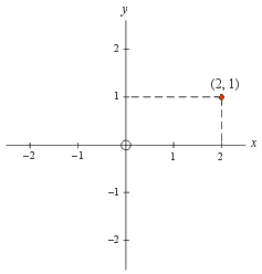Any point on the cartesian plane can be located by giving its horizontal distance to the right of the origin (this is called its x coordinate) and its vertical distance above the origin (this is called its y coordinate). For example the red dot in the cartesian plane shown to the right has an x coordinate of 2 and a y coordinate of 1. Sometimes we say that this point is at x = 2 and y = 1 but most often we use the ordered pair notation (2, 1) to describe this point. (Note that the number before the comma is always the x coordinate and the number after the comma is always the y coordinate.)

This method of using an x value and a y value to locate a point in the plane is called the rectangular coordinate system (notice the dotted rectangle shown in the picture). Another coordinate system in common use, for example for complex numbers, is the polar coordinate system; it uses a distance from the origin and a direction to locate a point.

Identifying points on graphs

We saw above that giving an x coordinate and a y coordinate locates a point in the cartesian plane. But we can turn the logic around: we could say that a point in the cartesian plane represents the simultaneous values of two quantities x and y. This interpretation is very important in science and technology where x and y can represent almost any quantities.

The following examples show how to identify points on progressively more complicated graphs.

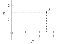Example 1: This graph has several features beyond what was explained above:

In this graph the horizontal axis is called p and the vertical axis q. Thus points on this graph represent values of p and q.
The labels p and q are sometimes written beside the axes rather than at their ends.
Only quadrant 1 was drawn, presumably because there is nothing interesting to show in the other quadrants.
The horizontal position of point A is half-way between p = 2 and p = 3. This mean that p = 2.5. Similarly, the vertical position of point A is half-way between q = 1 and q = 2. Thus point A is at p = 2.5 and q = 1.5.

(Actually the fact that p is midway between 2 and 3 means that p = 2.5 only because the horizontal scale is linear, which means that a movement of, say 1 centimeter, in the horizontal direction represents the same change in the horizontal quantity anywhere on the graph. There are other types of graphs such as logarithmic graphs where this is not true.)
In ordered pair notation, point A is at (2.5, 1.5). Be careful! This ordered pair does not mean x = 2.5 and y = 1.5; rather it means p = 2.5 and q = 1.5.

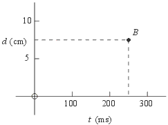
Example 2: The labels on the axes now have units. The label t (ms) means that t is measured in milliseconds and the label d (cm) means that d is measured in centimeters. Thus point B is at t = 250 ms and d = 7.5 cm. Graphs with units appear often in scientific or technical applications.

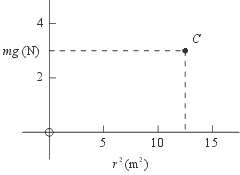
Example 3: The quantities plotted horizontally and vertically are now algebraic expressions. Thus at point C, the quantity mg has a value of 3 Newtons and the quantity r² has a value of 12.5 square meters.

Graphs with expressions on the axes appear often in scientific or technical applications. Their use makes it possible to transform a curve into a straight line, which is much easier to analyze.

6.2 - Linear functions and straight lines

Linear functions

Click here to review functions. Linear functions are the simplest of all the types of functions. A linear function takes a number x as input and returns the number m x + b as output:

m and b are constants. In words, x gets multiplied by m (this is called a scaling by factor m) and then gets b added on (this is called a shift by an amount b). Using function notation the linear function looks like this:

f (x) = m x + b.

If we let y = f (x) then it looks like this:

y = m x + b.

This is called the equation of a straight line because if we plot the points that satisfy this equation on a graph of y versus x then, as we will see below, the points all lie on a straight line.

A typical use of a linear function is to convert from one set of units to another. A simple example is if i is a distance measured in inches and c is the same distance measured in centimeters; then c = 2.54 i. This is just a scaling. A more complicated example is if c is a temperature measured in celsius degrees and f is the same temperature measured in fahrenheit degrees; then f = 1.8 c + 32. This is a scaling and a shift.

The equation of a straight line

In section 6.1 we introduced the cartesian plane with an x axis drawn horizontally and a y axis drawn vertically. Suppose that m and b are constants. We wish to graph the linear function:

y = m x + b,

on this plane and show that the graph is a straight line. To do this we make the following table of values of y (that is, of the expression m x + b ) versus x:

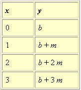
Notice the following:

Each row of the table gives a point on the graph.
One of the rows says that when x = 0 then y = b. Thus the point (0, b) is a point on the graph. Because this point lies on the y axis, the number b is called the y intercept.
As we proceed from one row of the table to the next, the value of x increases by 1 and the value of y increases by m. Because the increase is steady, the points must lie on a straight line and not some other curve.
The larger m is, the faster y increases. If m is negative then the value of y actually decreases. The number m is known as the slope.
x does not have to be an integer - it can be any real number. Because the real numbers are dense the graphed points are infinitely close together and form a solid line (i.e. there are no gaps).

Conclusion: The equation

y = m x + b,

where m and b are constants, is the equation of a straight line. m is called the slope and b is called the y intercept. This form of the equation is called the slope-intercept form. There are other possible forms; click here to see them.

Finding the equation of a straight line

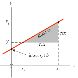
Given the graph of a straight line, there are several ways to find its equation.

Method 1: This method works only if the y intercept is visible.

Find any two points, (x₁, y₁) and (x₂, y₂), on the line and substitute their coordinates into the following formula to get m:
Get b from inspection of the y intercept of the graph.
Substitute the numbers that you have obtained for m and b into the equation y = m x + b.

Method 2: This method works even if the y intercept is not visible.

As in method 1, find any two points, (x₁, y₁) and (x₂, y₂), on the line and substitute their coordinates into the following formula to get m:
Substitute the number that you obtained for m into the equation y = m x + b. Also, take one of the points, say (x₁, y₁), and substitute its coordinates into the equation. This gives:
y₁ = m x₁ + b
It may not look like it, but this equation has only one variable, b, and you can easily solve for it.
Substitute the numbers that you have obtained for m and b into the equation y = m x + b.

Method 3: This method has the advantage that it uses only algebra, not geometry, and can be applied to any type of function, not just the straight line:

Find two points, (x₁, y₁) and (x₂, y₂), that are on the line. Take the first point, (x₁, y₁), and substitute it into the straight line equation, y = m x + b. This gives:
y₁ = m x₁ + b
Similarly, take the second point, (x₂, y₂), and substitute it into the straight line equation, y = m x + b. This gives:
y₂ = m x₂ + b
Together, these two equations constitute a system of two equations in the two unknowns, m and b. We can solve them for m and b using the elimination method. To be specific, if we subtract the first equation from the second, then b is eliminated and we get the equation:
y₂ − y₁ = m x₂ − m x₁,
which, when solved for m, gives the same equation as in the other two methods, namely:
Find b by back-substitution. To be specific, substitute the number that you obtained for m into one equation of the system of equations, say into y₁ = m x₁ + b. It may not look like it, but this equation has only one variable, b, and you can easily solve for it.

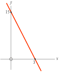Example: Use method 1 to find the equation of the straight line in the graph to the right.

Solution: Two points on this line are (x₁, y₁) = (0, 15) and (x₂, y₂) = (3, 0). Substituting these coordinates into the slope formula gives

= −5.

By inspection the y intercept is

b = 15.

Substituting these two values for m and b into the straight line equation, y = m x + b, gives

y = −5 x + 15.

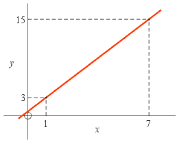Example: Use method 3 to find the equation of the straight line in the graph to the right.

Solution: Two points on this line are (7, 15) and (1, 3). Substitute the coordinates of the point (7, 15) into the equation of the straight line, y = m x + b, and then do the same thing for the point (1, 3). This gives a system of two equations in the two unknowns, m and b. Unknown b can be eliminated by subtracting the equations:

Solving for m gives m = 2. Backsubstituting m = 2 into, say, the first equation, gives 15 = 7 · 2 + b, which is easily solved to give b = 1. Substituting these two values for m and b into the straight line equation, y = m x + b, gives

y = 2 x + 1.

6.3 - Other types of graphs

Literally dozens of different types of graphs (or charts or plots) have been invented. We will describe the three types that the Algebra Coach uses. We will assume that the variables of interest are called x and y and that we want to plot the graphs on the cartesian plane.

Graphs of functions

A function can be described as a machine that takes a number x as input, and applies some rule to it that gives a corresponding number y as output:

This means that we can make a table of values of the function. This is a two column table whose first column is a list of x values of our choosing, and whose second column is the corresponding y values calculated using the function rule. (The x values should be uniformly spaced and they should be in order from smallest to biggest. Click here to see an example.)

We can then plot the table of values. Each row of the table becomes a point on the graph. If the function is not varying too rapidly then we can connect each point to the next one with a straight line segment. If the x values are chosen close enough together then the sequence of straight line segments will appear to be one smooth curve.

Notes:

The graph of a function can have only one y value for any given x value.
The Algebra Coach uses this table of values technique to plot functions.
Click here to see graphs of various types of functions.

Graphs of relations

A relation is simply an equation containing the two variables x and y, but that has not necessarily been solved for y. An example is the general form of the equation for the straight line

2 x + 3 y + 4 = 0.

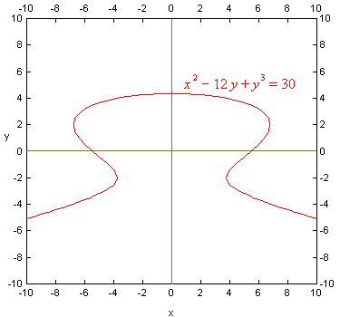
If a relation can be solved for y, then we again have a function which can be plotted as described above. For example the relation 2 x + 3 y = 4 can easily be solved for y. However, many relations can’t. An example is the relation

x² − 12 y + y³ = 30,

which is graphed to the right. The problem is that if we can’t solve for y then we can’t make a table of values.

Thus we use a totally different approach; we systematically test every point of the cartesian plane (or every pixel on the computer screen) to see if the x and y values at that point satisfy the relation. If they do then we plot a point there; otherwise we don’t. The set of all points that satisfies the relation is called a locus of points and for this example the locus of points is a curve. Obviously testing every point in the plane would take forever but there are approximate methods that allow it to be done quickly.

Notes:

The Algebra Coach uses such an approximate method to plot relations.
Unlike the graph of a function, the graph of a relation can have more than one y value for a given x value.
You may be familiar with topographical maps. These are maps that show the elevations of mountains, valleys and other geographical features by using contours, which are lines of constant elevation. The graph of a relation can be though of as a contour on a contour map. Here is an example showing why:
- Create a function of two variables from the left-hand-side of the above relation, like this:
  f (x, y) = x² − 12 y + y³.
  This function takes two numbers, x and y, as input; evaluates x² − 12 y + y³; and returns that number as output. For example if x = 5 and y = 2, then the function calculates f (5, 2) = 5² −12 · 2 + 2³ = 9, and returns the number 9.
- Now imagine that x and y are the longitude and latitude of a location and that the output of the function is the elevation at that location. For example at x = 5 and y = 2 the elevation is 9.
- Then finding all x and y that satisfy the relation
  x² − 12 y + y³ = 30
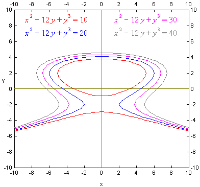  can be interpreted as finding the contour whose elevation is 30.
  
  The graph to the right shows four contour lines at elevations of 10, 20, 30 and 40 for our function of two variables.

Parametric plots

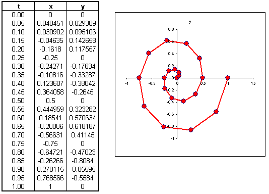
A parametric plot is a completely different way to draw a curve. Let (x, y) denote a point along the curve. The idea is to let both x and y be functions of a new variable or parameter, usually called t. You can arrange it so that when t = 0 you are at one endpoint of the curve, when t = 1 you are at the other endpoint of the curve, and as t ranges from 0 to 1 you move along the curve from one endpoint to the other. You could imagine that t represents time and that as time progresses you move to different points along the curve.

Example: Let

x (t) = t · cos (4 π t),
and
y (t) = t · sin (4 π t),

be the x and y coordinates of points along a curve, expressed as functions of a parameter t. The 3-column table of values below shows values of x and y as the parameter t ranges uniformly from 0 to 1 in 20 steps. The points in the parametric plot to the right are the 21 values from the table. They have been connected with straight line segments. (Using smaller increments of t would have resulted in a smoother curve.)

If t denotes time then the curve could describe the path of an object that starts at the origin and spirals outward, slowly at first, and then ever more quickly (as evidenced by the fact that the dots are getting farther apart).

Another nice example is the cycloid.

Using graphs to solve equations

Many equations cannot be solved using algebra. To solve these we must resort to approximate methods involving graphs and computers. Here is the process:

Prepare a function corresponding to the equation:
Let the unknown be called x. Use algebra to move everything over to the right-hand-side of the equation. This puts the equation into the form 0 = f (x), where f (x) denotes some expression involving x. Now replace the 0 on the left-hand-side by the variable y. The result is y = f (x), ie. y is some function of x.
Graph the function and estimate the roots:
Make a graph of the function y = f (x), plotting y vertically versus x horizontally. Find the points where the function crosses the x axis. These are the values of x for which y = 0 or f (x) = 0. In other words, these are the required roots of the equation. Thus from the graph we can find the number of roots and their approximate values.

Example: Consider the equation

. Find the number of solutions and their approximate values.

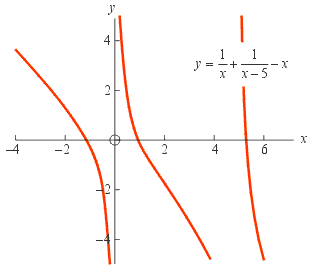
Solution: The first step is to prepare the function. Bring everything to one side of the equation. There are many ways that this can be done. One way is to simply subtract x from both sides of the equation to get:

Then replace the 0 on the left-hand-side by y:

The second step is to graph this function, as we have done to the right. The roots are the points where y = 0 (i.e. the x intercepts). The graph shows that there are three such points, approximately at

x = −1, x = 1 and x = 5.2

Note: Another way to prepare the function is by first clearing denominators in the equation by multiplying through by x (x − 5):

then distributing

x³ − 5 x² = (x − 5) + x,

and then bringing everything to one side of the equation:

x³ − 5 x² − 2 x + 5 = 0.

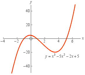Now replace 0 by y and graph the function:

y = x³ − 5 x² − 2 x + 5,

as we have done to the right. This cubic function looks completely different from the previous function but crosses the x axis at exactly the same points. Thus we find the same three roots for the equation; namely x = −1, x = 1 and x = 5.2 (approximately).

One problem with multiplying through by x (x − 5) is that this can introduce extraneous roots. Therefore we must check our solutions by substituting them back into the original equation.